LMS: Let the Model Self-Adjust

No, that is not really what LMS stands for. But why not?

Previous articles have discussed what a linear state model is, and how a dynamic state transition model can be constructed. Whatever method was used, when you go back to validate the model's results, you might find the result disappointing.

In situations like this, wouldn't it be nice to say:

That is the topic for this installment.

 

Introducing LMS adaptive tuning

A method for doing this kind of parameter adjustment is the LMS method.^[1] The ideas are quite easy to implement, and easy to understand too, as long as you don't let notations for all of the "adjustable constants" confuse you. However, in the interest of full disclosure: the simplicity comes at the expense of speed. You will need plenty of data and plenty of patience.

Start from the basic linear state model equations, as they exist after your initial attempts at model construction.

$$\begin{array}{c}{\stackrel{‸}{x}}^{i+1}=A{\stackrel{‸}{x}}^i+B{u}^i\\ {\stackrel{‸}{y}}^{i+1}=C{\stackrel{‸}{x}}^{i+1}\end{array}$$

Collect data from actual system input/output measurements. This will be covered in more detail in a future installment. But for now, let us just presume that the data set has reasonable if somewhat noisy measurements of system input and output values over an extended interval of time.

Apply the input data to the mathematical model, term by term. This allows the model to develop a sequence of estimated next-state vectors x for each point, and from these, the predicted output values y.

The predictions generated by the model can be compared term-by-term with the output values the system actually produced. Identify the model prediction errors as the differences between what the model projects and what the actual system does:

Δ yi+1 = [projected y]i+1 - [actual y]i+1.

The LMS strategy for adjusting the values of parameters (that are eligible for adjustment) can be summarized as follows:

Don't panic! This is much easier than it first sounds. It just means that you make a lot of very small pushes in the right general direction at every point, as you go. We will now examine details of how to do this for each part of the system model.

 

LMS Adjustments to Observation Matrix

Suppose there is low confidence in the values of the output observation matrix terms.

Consider the consequences of making an adjustment to the C matrix terms according to the following formula, where the update gain coefficient α is very small. The x vector is the current estimated state vector. The hat notation on the C matrix indicates the original estimated values for these parameters.

$$C\leftarrow \stackrel{‸}{C}+\alpha x^T$$

After modifying the output observation matrix in this manner, the new output calculation will produce the original output value plus a small adjustment.

$$\left(\stackrel{‸}{C}+\alpha x^T\right)x=\stackrel{‸}{C}x+\left(\alpha x^T\right)x=\stackrel{‸}{C}x+\alpha \left(x^{T}x\right)$$

The xTx term is a sum of squares and always positive. Thus, choosing the α gain constant to have the negative of the sign of the model prediction error will have the effect of reducing the prediction error at the current point.

By including the current output prediction error in the updating formula explicitly, it is possible to guarantee that the adjustment is proportional the current output error but opposite in sign. Pick the α constant to be small and positive, then make each correction as follows.

$$C\leftarrow \stackrel{‸}{C}-\alpha \text{Δ}y{x}^T$$

For cases when C has multiple rows, just repeat this for each of the rows of C, one at a time. The adjustments for each of the output variables can use a different value of the α gain constant. To make this somewhat easier to manage, reorganize the various gain constants as a diagonal matrix λ with terms somewhat larger or smaller than 1.0 to control the relative learning rates on each individual term, while scalar α provides an overall rate adjustment for all output variables.

$$C\leftarrow \stackrel{‸}{C}-\alpha \text{Δ}y{x}^T\lambda$$

What happened to the fancy talk about "approximation to the local gradient?" Well, we got that almost for free, because the value of the state estimate x serves as this local gradient estimate.

You might also wonder about the effects of noise. The model will of course generate results that are not subjected to the same noise disturbances that affect the real system. Since the "prediction errors" depend directly on the noisy outputs from the actual system, wouldn't using these noisy values cause the corrections to chatter upward and downward? Yes, and if the adjustments are too large, the process never gets anywhere. But make every adjustment very small — in fact, microscopic — and over an extreme large number of very small updates, truly random effects will balance out very close to zero, while non-random effects will nudge the model parameters consistently toward improved values.

You don't need to change all of the output parameter values just because you could. Some adjustments would not be reasonable. For example, sometimes you know that the model includes some states that are not directly observable, and therefore have a zero parameter term in the C matrix. The adjustments should not be allowed to change the zero observation matrix term into something that is non-zero.

 

LMS Adjustments to Input Coupling

Now let's consider adjustments for the parameters in B, the input-coupling matrix, taking one input value and one output value at a time. Using the lessons learned when examining the C matrix adjustments, propose an adjustment to the B matrix terms according to the following.

$$B\leftarrow \stackrel{‸}{B}-\alpha \text{Δ}y{C}^{T}u$$

Substitute this adjusted value of the B matrix into the state transition equations. We again see that the results consist of the previous state projection, plus a very small correction.

$${\stackrel{‸}{x}}^{i+1}=A{\stackrel{‸}{x}}^i+\left(B-\alpha \text{Δ}y{C}^T{u}^i\right)u^i$$ $$=A{\stackrel{‸}{x}}^i+B{u}^i-\alpha \text{Δ}y{C}^T{\left(u^i\right)}^2$$

Let's see what happens when this small adjustment affects the next state prediction and is observed with the C matrix.

$$C·-\alpha \text{Δ}y{C}^T{\left(u^i\right)}^2=-C{C}^T\alpha \text{Δ}y{\left(u^i\right)}^2$$

Since the two squared terms always yield positive scalar values, we are guaranteed that the adjustment will reduce the model's output error at the current point.

As was the case for the C parameter updates, the sign is critical to the algorithm. Each term of the B matrix, even each individual update, could use a different adjustment multiplier, as long as the result is small and of the correct sign. We again let λ multipliers represent the differences in scaling between different B matrix terms, and leave an α scalar controlling the overall update rate. This is the new adjustment formula for updating the input coupling matrix terms.

$$B\leftarrow \stackrel{‸}{B}-\alpha \text{Δ}y{C}^T\lambda u$$

Because of the CT term in the updating formula, the most vigorous adjustments go toward adjusting parameters associated with states that have the strongest influence on the output variable. That could be a very good idea, but maybe not in special cases where you are trying to adjust secondary effects rather than the main ones. As said before, it is not the value of the terms but the sign that is critical, so an alternative updating formula that influences all terms more uniformly is

$$B\leftarrow \stackrel{‸}{B}-\alpha \text{Δ}y{\mathrm{sign(C)}}^T\lambda u$$

As in the case of the output matrix updates — don't use it if the changes the updating formula suggests are not appropriate for your model form.

 

LMS Adjustments to State Transition Matrix

Finally, let's consider adjustments for the state transition matrix terms A, the heart of the model. This turns out to be very similar to the other two cases.

Propose an updating formula with the following form.

$$A\leftarrow \stackrel{‸}{A}-\alpha \text{Δ}y{C}^T{x}^T$$

Substituting this adjustment into the model equations:

$${\stackrel{‸}{x}}^{i+1}=\left(\stackrel{‸}{A}-\alpha \text{Δ}y{C}^T{\stackrel{‸}{x}}^{iT}\right){\stackrel{‸}{x}}^i+B{u}^i=\left(\stackrel{‸}{A}{\stackrel{‸}{x}}^i+B{u}^i\right)-\alpha \text{Δ}y{C}^T\left({\stackrel{‸}{x}}^{iT}{\stackrel{‸}{x}}^i\right)$$

The effects on the observable outputs are then:

$$C·-\alpha \text{Δ}y{C}^T\left({\stackrel{‸}{x}}^{iT}{\stackrel{‸}{x}}^i\right)=-\alpha \text{Δ}y\left(C{C}^T\right)\left({\stackrel{‸}{x}}^{iT}{\stackrel{‸}{x}}^i\right)$$

Once again, the squared terms produce non-negative scalar values, and we can be sure that the incremental adjustments to the state transition matrix are always in the direction of improvement.

Referring back to the discussion regarding updates to the input coupling matrix B, an alternative updating scheme that does not favor the state equations contributing the most directly to output observations is the following.

$$A\leftarrow \stackrel{‸}{A}-\alpha \text{Δ}y{\mathrm{sign(C)}}^T{x}^T$$

As in the case of the other model terms, there are options to control the relative adjustments applied to each state variable. Let P represent any positive definite matrix. To avoid confusion with the rate adjustment factors, select the P matrix so that the norms of row and column vectors are not too far away from 1.0. This matrix will have the property that for any vector v:

$$v^{T}Pv>0\text{when}v\ne 0$$

Modify the update expression to include an additional P matrix as a "mixing" term, and then take a look at changes in the observable outputs.

$$A\leftarrow \stackrel{‸}{A}-\alpha \text{Δ}y{C}^T{x}^{T}P$$

 

$$C·-\alpha \text{Δ}y{C}^T\left(x^{iT}P{x}^i\right)=-\alpha \text{Δ}y\left(C{C}^T\right)\left(x^{iT}P{x}^i\right)$$

Thanks to the properties of positive definite matrices, the sign on the incremental change remains correct, so the adjustment is guaranteed to produce gradual improvement in the output prediction error. This tells us that there are many ways of adjusting the transition matrix terms successfully. The advantage of the P transformation is that it allows adjustments to be "spread around" to parameters having no direct and immediate influence on output terms.

Some common strategies for selecting a P matrix:

• Let the P matrix to be an identity matrix. This reduces to the original case without the "mixing" terms.

• Choose the P matrix to be a diagonal "scaling" matrix with all positive terms. This could help to keep adjustments consistent with sizes of expected state variable variations.

• Choose the P matrix so that it has approximately 1.0 terms on the main diagonal, and small, unbiased random terms off diagonal. This kind of "annealing" might help to break up artificial patterns in the update sequence and produce improvements that might otherwise be difficult to discover.

• Choose the P matrix to be the inverse of the state covariance matrix. An estimated covariance matrix can be obtained from the x state sequence calculated by the model; then invert this matrix. When certain state variables are relatively noisy and others are relatively quiet, this "levels the playing field" so that corrections are applied roughly in proportion to how trustworthy the current state estimates are.

Clearly, different values of P will send the adjustments along different trajectories. Since the state space representation is not unique, you can never be sure of exactly how your model might change — but you can expect improvement.

As with cases before, do not apply changes to terms that are not supposed to change. For example, if your state transition matrix is supposed to have a diagonal structure, do not change off-diagonal terms.

 

Adjust everything all at once?

There is nothing that says you can't try it. But keep in mind that the linear models are not unique, and things could rattle around for a very long time, producing relatively large adjustments to the model but no improvements of any significance in results.

 

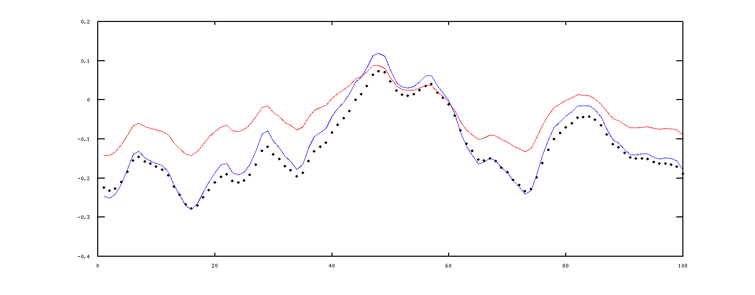
An illustration

As a credibility test, the LMS method was applied to a linear system with a randomized single input and a single output. In theory, it should be possible to match this closely, except for the hidden random errors within the real system state variables. The black dots in this plot show the output values observed from the system. The red curve shows the output trajectory predicted by the initial model... not so good. The blue curve shows the response after the LMS algorithm has performed 100000 updates. Not perfect, but much better.

We will revisit this topic later in the series, but there are a few more things we need to know about first.

 

---