Test Case: Identifying States in Correlation

Last time we discovered that the telltale signs of states are patterns in correlation data that look very much like exponential impulse response sequences the system produces. Let's see where this leads us.

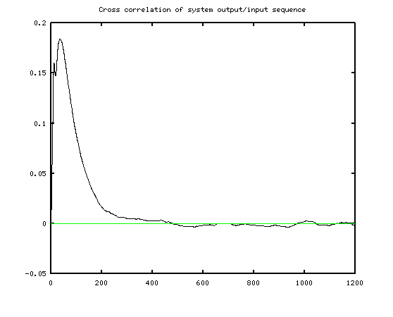
An experiment that produced 500000 input/output sample pairs was performed. As discussed in previous installments, correlation analysis was performed to determine estimates of the input-to-output cross correlation and output-to-output autocorrelation sequences. Here is what the curves looked like.

Crosscorrelation:

Autocorrelation:

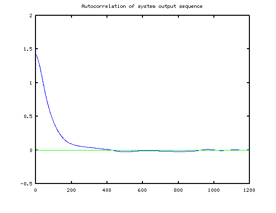
These are quite similar. Let's see what evidence of system states we can find in the cross-correlation sequence.

 

The major exponential feature

The crosscorrelation features a shape that looks broadly like an exponential decay. Using the highly sophisticated search method known as "hack and try," I constructed an exponential function and tweaked the amplitude and decay rate parameters looking for something that seemed to match. I settled on on:

  pat1(iterm)=0.355*exp(-iterm/70); 

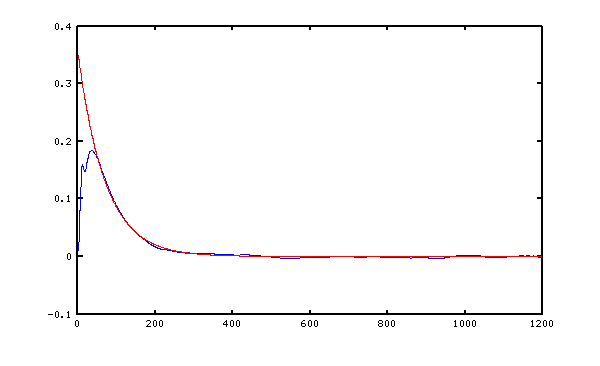
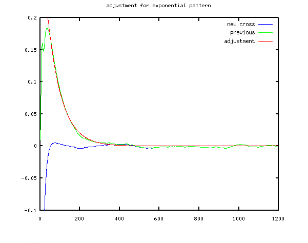
Removing this curve from the original correlation data makes it a little easier to see what other patterns are left. The adjusted curve is shown below in blue.

  crosscorr = crosscore - pat1;

 

A small oscillation?

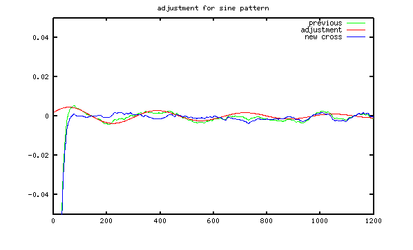
There is an up-down patterns that looks like a small sine wave oscillation, with not very much damping. Again using more luck than science, I approximated as follows.

  pat2(iterm) = sin(2*pi*iterm/330+0.4)*0.0050* exp(-iterm/700); 

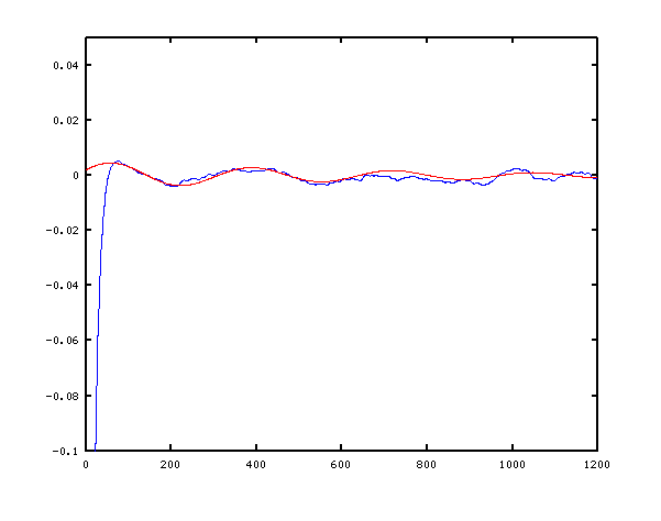
This response pattern is also removed, leaving adjusted curve again shown in blue.

  crosscorr = crosscore - pat2;

 

A fast exponential

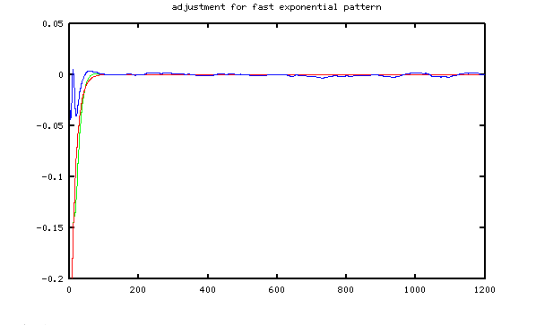
There is a relatively fast exponential response pattern at the beginning of the correlation curve. It is completely settled and gone in about 70 samples, starting negative and then decaying upward to zero.

  pat3(iterm)= -0.330*exp(-iterm/14); 

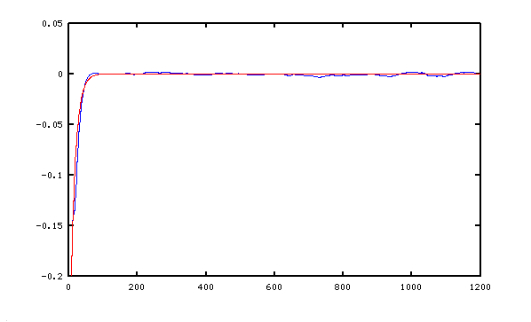
After this pattern is removed, what remains is shown in blue below. There is not much left to see besides a small, fast disturbance near 0. Is that real? It seems like the duration is a little too long to be a test signal artifact, but it doesn't seem like a feature that I want in the model, so for now I'll choose to disregard it.

 

Accounting time

There were three identified patterns to be retained. Let's combine them and compare to the original correlation curve.

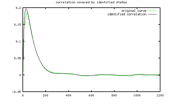
Each of the exponential patterns is related to one state. The oscillation is associated with two states. So a four-state model should be capable of representing this system sufficiently.

The correlation analysis should be repeated for each output. All of the outputs will be affected by the same state response patterns. However, some outputs could have very weak connections to some of the states, while those effects show up prominently in other outputs. If evidence of significant additional states shows up, add to the state tally for representing the system.

 

Where to next?

At the expense of some time for exploration and hacking, some useful information revealed itself about order the model needs to be to represent the system. Our analysis is finished.

But some additional information did happen to fall out of this analysis, some numerical estimates. Is it possible to leverage these to set up a model directly? It probably wouldn't be very good, but that would at least provide some evidence to support the validity of the analysis. Next time, we will take a further look.

 

---