State Observers: Theory

After obtaining a dynamic state transition model, it is can be used by applying input value over a sequence of time steps, and updating values of the hidden internal state variables. From the accumulated information, it is able to produce predictions of what the system output is expected to be.

The limitation of this approach is that it is somewhat divorced from reality. To understand what that means, let's perform two simulations using the model. In the first simulation, apply the original input sequence, and observe the sequence of output predictions. Then, for the second simulation, add about 4% zero-mean uniform random noise into each state variable after each update. The second simulation won't be an exact prediction of anything, but it will illustrate the kind of effects to expect.

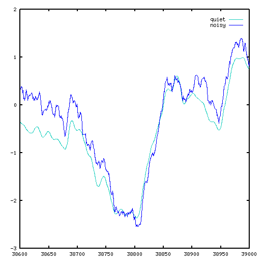
Over time, the noise effects become integrated into the state of the model, and some significant differences result. If noise produces stray displacements of something like 20 percent or more, it becomes difficult to determine meaningful model parameter adjustments, and the model results can degenerate to irrelevance.

 

Models and state estimation

The problem with operating the model as we have done previously is that it is a little divorced from reality. The model predictions are completely separate from what the system is actually doing. If the model predictions are actually proving to be quite wrong, the model has no way to know that, and it will continue along the trajectory that the erroneous state information implies.

So, suppose we formulate a different kind of problem. Assume that the system model is known and capable of making highly accurate predictions — provided that it has highly accurate estimates of the system state variables. In this alternative problem, the goal is to use all available information about the system inputs and outputs to produce the best possible estimate of the state variable values. This is called the state observer problem.

The state transition equations and the state observer equations are in some respects analogous to open loop and closed loop control strategies from control theory. With an open loop strategy, you know from past studies how your system is going to respond to a given input signal, so the best control strategy is to apply the known input signal that will take your system from its initial state to the target state. Does the system actually get there? Probably not, but close enough to make this strategy very useful. With a closed loop strategy, you observe the actual system output, compare it to what the system output should be, and based on this, apply a feedback adjustment to incrementally correct the discrepancy. The two strategies can be applied together to form a powerful combination.

 

State observer equations

We are going to start getting a little more formal now. Observer equations are a set of equations that attempt to deduce from the system input and output sequences what the best estimated values of state variables are. As you can imagine, the relationship between the observer equations and state transition equations is close, and we want to take advantage of the known state transition equations as much as possible. The system state transition equations governing the linear system are:

$$x_{k+1}=A{x}_k+B{u}_k+v_k$$

where

The associated output observation equations specify how hidden states produce observable output values.

$$y_k=C{x}_k+D{u}_k+r_k$$

where

Though model matrices A, B, and C, are presumed known from the state transition equations, the state variable values and the random disturbance values are not known. The new state observer problem is to select observer matrices E, F, and G that define a new state observer equation dynamic system to be determined. All state variables of this system are completely observable, and they provide estimates of the values of the system state variables.

$$z_{k+1}=E{z}_k+F{y}_k+G{u}_k$$

where

Noise effects are not involved. It can be noted that the values of the observer state variables z and the transition state variables x in the state transition equations mean the same thing, only produced in two different ways. If these ways were somehow made completely consistent, the z and x would be exactly the same except for some small residual noise effects.

Suppose that the state variable estimates and the actual states are initially different. The tracking error in the observer equations is the vector difference between observer-estimated state values and the hidden actual state values. If the design is successful, and the modeling is perfect, the observer equations will over time produce state estimates that converge to the correct system state values.

Start with the expression for the state observer's tracking error, the difference between the estimate produced by the observer and the estimate predicted by the state transition equations. If these are consistent, these two estimates will match exactly. But if they are not consistent — the side effects of the unobservable noise affecting the actual state transitions — we want to drive this difference to zero as closely as possible.

$$z_{k+1}-x_{k+1}\to 0$$

Make the following subsitutions.

 

$$z_{k+1}-x_{k+1}=E{z}_k+F\left(C{x}_k+D{u}_k\right)+G{u}_k-A{x}_k-B{u}_k$$

 

$$z_{k+1}-x_{k+1}=E{z}_k+\left(\left(,FC-A,\right)\right)x_k+\left(\left(,FD+G-B,\right)\right)u_k$$

 

Make the following design selection.

$$G\equiv B$$

Establish a structure of matrix F so that the following constraint is satisfied.

$$FD\equiv 0$$

This is usually trivial to accomplish, by setting a few selected terms of F equal to zero. (In general, any nonzero D terms are undesirable because they mean direct instantaneous input-to-output coupling. In the typical case where the D matrix is already zero, this restriction becomes moot.)

In combination, these design constraints eliminate the term related to input uk .

Now make the following selection for observer equation matrix E.

$$E\equiv A-FC$$

Substituting this into the previous expression for state estimation error yeilds

$$z_{k+1}-x_{k+1}=\left((,A-FC,)\right)\left((,z_k-x_k,)\right)$$

and thus

$$z_{k+1}-x_{k+1}=E\left((,z_k-x_k,)\right)$$

If the (A - FC) matrix is stable, the sequence of tracking errors reduces exponentially to zero, which means the estimate values for the state converge to the actual state values. The stability can be guaranteed if the adjustable terms of matrix F are selected in such a manner that

$$\parallel E\parallel {}_{\text{σ}}<1.0$$

The sigma notation indicates the "spectral matrix norm." This simply says that the magnitudes of all the eigenvalues for the matrix (in general complex) must be less than than 1.0. ^[1]

For a stable system, the condition is satisfied trivially by initially setting the F matrix to have all zero terms. This trivial choice is also a very poor one, however, so start improving it incrementally, by tweaking the terms of F until you get the kind of steady convergent behavior that you want. Just make sure that your adjustments do not cause any eigenvalues to become too large. This cut-and-try process is not elegant, but using an appropriate software tool to assist with computing the eigenvalues, it is not difficult.

So much for the theory. Next, we will give this process a try, setting up observer equations and tuning the F matrix design for system equations we have seen previously to give the observer matrix E desirable properties.

 

---