State Observers with a Weak Model

We saw last time the ability of the observer to produce improved state estimates. Well, at least we saw this indirectly. The output is derived from the state, and the states were adjusted to improve output tracking, and the output tracking was clearly better. So the natural conclusion is that the state estimates must be pretty good, right? Well, not necessarily. The two goals, representing system states accurately and tracking the system output accurately, are not necessarily the same thing. It is important to understand the difference.

Let's see what happens if the output observer technique is used with a model that is known to be badly compromised. We will obtain this by starting from a model we think is reasonably good and deliberately compromise it.

 

Making a weak model worse

In the previous installment, we had a sixth-order system worked pretty well, though not perfectly, in its attempts to represent system behaviors. That model is now deliberately degraded, in the following manner.

1. The model had two states that were decaying exponentials with opposite sign and similar magnitude. We will disable the one that decays over a longer period of time.
2. Discard the oscillatory mode with the longer decay period.
3. Retain the oscillatory mode with the quicker decay period, but round the values of its output observation coefficients.

This is not scientific. The model ends up with an oscillatory mode that was almost excluded from the model at the outset, and one decaying mode with an output observation term that is rather hypothetical. This should not be expected to perform particularly well. And of course, I will do nothing to verify that any of the ad-hoc adjustments are valid. Here is the degraded model.

 
Amat = [ ...
     0.93000,   0,         0  ; ...
     0,         0.925,   -0.300; ... 
     0,         0.295,    0.920  ];

Bmat = [ 1; 1; 0];

Cmat = [ 0.12, -0.015,   0.004 ];

The highly scientific cut-and-try approach illustrated in the previous installment was used again to design the observer gain matrix F: try, test, tweak — and repeat. The design restriction required for stability was the following.

$$\parallel A-FC\parallel {}_{\text{σ}}<1.0$$

Here are the locations of the eigenvalues before introducing any state observer feedback terms.

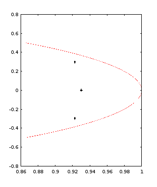
Here are the locations of the eigenvalues before introducing any state observer feedback terms.

For observer gain adjustments that are not too slow but not too sensitive to residual noise effects, the eigenvalues were adjusted to have magnitudes in the range 0.94 to 0.97.

I eventually settled on the following observer gain matrix.

Fmat = [-0.33; 1.2; -2.4 ];   % Shifts middle eigenvalue pair 

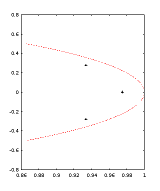
Here are the locations of the eigenvalues after the observer gains are applied.

These are the eigenvalues for these observer gains.

evec =
   0.97495 + 0.00000i
   0.93363 + 0.27929i
   0.93363 - 0.27929i

magnitudes =
   0.97495   0.97451   0.97451

 

Simulation: deficient model with state observer

Time to run the experiment. At each step, apply the input data to the stripped-down system state equations to predict the next system output. Then, use its state observer to calculate adjusted state estimates for better output tracking.

Let's go straight to the bottom line. Here is a plot comparing the output predictions for the deficient model plus state observer to the noisy output observed from the actual full-rank system.

 

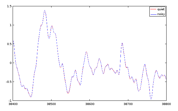
How is this possible? What does it mean?

It is hard to claim that the state representation is particularly accurate, given that some of the states are missing entirely. Clearly, as the state transition equations supply less accurate information, the state observer equations are working harder to make up the difference and maintain the quality of the output tracking.

The lessons here are:

1. If the purpose of the modeling is to obtain best estimates of all the internal system states, corrections of the observer can obscure deficiencies in the state representation.
2. If the purpose of the modeling is to obtain improved predictions of the output sequence, the observer corrections can greatly compensate for inadequacies of the state transition model.

You need to use some judgment. But for applications in which the purpose of the model is to predict and track output sequences, it should be clear that using a state observer makes performance of the state transition model less critical. Anything somewhat reasonable is good enough.

How far can you take the simplifications? In the next couple of installments we will explore theoretical and practical sides of this question.

 

---