The Steady-State Kalman Filter

In the preceding installments, we observed that with reasonable observer gains, an observer system will undergo a transient period as it attempts to correct for the lack of knowledge about the initial state. But after that, the observer begins tracking more closely and the corrections are primarily to compensate for noise effects. If the noise sources are stationary and their variances do not change over time, the state variances settle. In the example case, the settling period was about 100 updating intervals.

When none of the terms going into the Kalman gain formula are changing, the Kalman gains are not changing either. What is the point in continuing the variance calculations when you know that nothing will change? The settled final value of the state variations is often called the steady-state variance. (That is, the noise model has settled. There is still plenty of bouncing around in the individual values of state variables.)

Steady-State Kalman Gains

When the Kalman gains settle, either to a steady constant value or to a bounded value that changes very little, you are probably better off to use the settled steady-state Kalman gains and dispense with the Kalman variance updates in your implementation. To determine the steady-state Kalman gains, you can simply evaluate the variance updating formulas for a sufficient number of cycles, so that there are no further significant changes, and this will provide a very acceptable approximation for the gain values.

We know that the steady state Kalman gains will not be the "best choice" until the system settles after the initial transient from an unknown starting state. Would this lack of optimality for a limited number of initial samples make any difference to your application? By giving up this slight edge in start-up performance, the simplifications are immense. In effect, you make these calculations once, off-line, and then hard-wire the results into your observer equations as a fixed set of gain values.

What is the cost?

Let's apply this idea for the example system we have be looking at in the last few installments. Here again are the parameters of the noisy system model.

And here are the formulas for calculating the optimal gains at each step, as discussed in the previous installment.

Let's fire up Octave and perform these calculations. The example appears to converge in about 100 update steps using a reasonable but non-optimal set of observer gains, so let's allow 200 repetitions.

  % Kalman gain updates
  Wmat = (Amat*Pmat*Amat')+Qmat;
  Xmat = (Cmat*Wmat*Cmat')+Rmat;
  KmatK = Wmat * Cmat' * Xmat^-1;
  Pmat = Wmat + KmatK*Cmat*Wmat + Wmat*Cmat'*KmatK' + KmatK*Xmat*KmatK';

Here is the steady state Kalman gains calculated.

 Kss = [  1.0000,  -0.4058,  -0.8606,  0.0000  ]' 

Off to the races...

Let us now repeat the simulation of the observer, but with three different sets of observer gains.

1. Manually tweaked observer gains that looked good.
2. Steady state Kalman gains, as calculated.
3. The full Kalman filter with dynamically adjusted gains.

And here's the finish line...

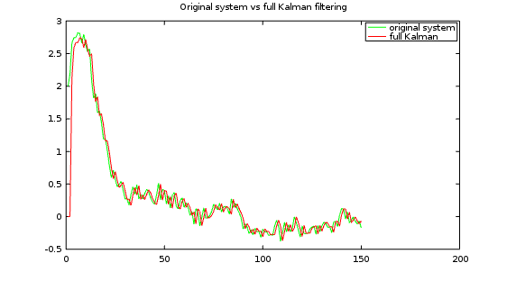
Comparing the Kalman observer to the original system. You can see that it tracks every change closely.

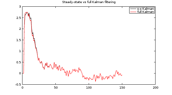
Comparing the complete Kalman observer to the Steady-State Kalman observer, the expected minor differences are visible in the initial transient, followed by the expected identical behaviors for all time following that. The Steady-State Kalman filter won't always work quite this well, but a lot of the time it does. This illustrates how pointless continuously recalculating the full Kalman Filter variance and gain updates can be.

Finally, let's see how my manually-tuned observer compares.

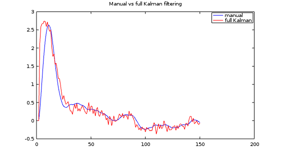
The manual observer clearly doesn't have the bandwidth to track the most rapid changes accurately, and it doesn't settle nearly as fast as the Kalman variations. However, let's consider whether this is a bad thing. The Kalman filter is intended to respond optimally for the full spectrum of random noise, but in my sampled data system I would prefer my model to disregard the band above 20% of the Nyquist limit. In effect, I happened to get low-pass data smoothing "for free." This more efficient processing might be more beneficial than theoretical optimality.