Considerations for Data Smoothing

A parallel question, while thinking about what a Kalman filter optimizes, is where an optimal result is needed. Optimal estimation problems are often classified as:

1. A filter problem. Given the input/output response data for the system up to time N, determine the optimal estimates at time N.
2. A predictor problem. Given the input/output response data for the system up to time N, determine the optimal estimates at time N+k, beyond the last position observed.
3. A smoother problem. Given the input/output response data for the system up to time N, determine the optimal estimates at time N-k prior to the last position observed.

Given what you already know about a Kalman Filter, and with a broad hint from its name, it is apparent that a Kalman Filter is truly...

A predictor, not a filter.

 

What does a Kalman Filter predict?

Consider the general form of the Kalman filter. Reviewing the general form of the Kalman Filter (separating the noise processes from the response produced by the driving input):

  forward projection step:    tn+1 = A xn 

  forward output prediction:  vn+1 = C tn+1
 
  observer correction:        xn+1 = tn+1 - K·(vn+1 - yn+1)

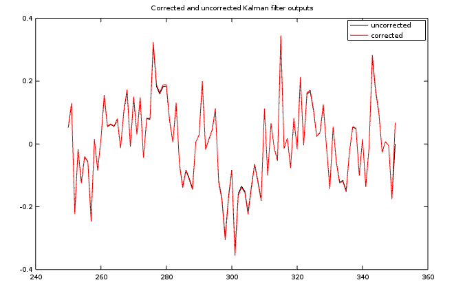
So it is clear that the final adjusted value is a best prediction of the next state vector value. Is that what you needed? Maybe, but probably not. Instead of the best estimate of state, you probably care more about the best estimate of the output. And the way to get this best estimate of the output is to take the corrected best estimate of the state and re-apply the observer equations.

  output calculation:         yn+1 = C xn+1

Ordinarily, a Kalman filter does not make this calculation^[1], because it does not need to. The Kalman filter process only need the predicted next output value. How much difference is there between the optimal prediction and the optimal filter value? As you can see in the following plot, the difference is often too small to worry about, but it might be worth taking a look.

 

What about the future?

Without formal proof, for balanced unbiased noise sources, the optimal projection of the state (and corresponding outputs) is the projection in which the noise disturbances are at their expected values. Or in other words, zero. Or in other words, all you need to do is apply the state transition equations for the number of steps you want to project ahead.

At first this seems implausible. The predictions couldn't possibly be very good, considering how the noise sources are going to send the system this way or that. But think of it this way. In the cloud of future possibilities, the multiple-step forward projection runs directly through the center of that cloud.

 

What about the past?

How do politicians typically score the most credibility points? By advocating a simplistic and conventional political doctrine and then dealing with the blowback when the truth comes out, for better or worse? Or by waffling and deflection, waiting until something positive happens, then claiming that this is what they had supported all along? As they say, hindsight has its advantages.

The same sort of principle applies in the case of Kalman Filtering. The predictions of the Kalman Filter are optimal for the case of looking one step into the future given what happened in the past. But couldn't the estimates at some particular point in time be a little better if they include future information as well as past information? You can maybe afford to do this if you are willing to wait a few steps to see what the future holds.^[2] That could yield better state and output estimates — by a little. This is known as Kalman Smoothing.

Typical Kalman Smoothing solutions perform their calculations in two sweeps. First, the ordinary Kalman Filter equations are used to best estimate the predicted next state values up to time N+K. Starting from the end of that sequence, the data are Kalman Filtered with a variant of the normal Kalman Filter equations moving in the reverse-time direction until reaching term N, where the final result is issued for that point.

If you are performing data capture first and then applying the Kalman Filter operations later offline, it is not so terribly expensive to continue the backward pass all the way to the start of the data set. For the case of dynamically changing covariances, you can retain the covariance matrices and Kalman gains for all of the back-steps, making them relatively less expensive.

You can skip the mathematical details if you wish, but there isn't anything very complicated here. Start with the best state estimate from the final step. Use the inverse of the state transition matrix to project this state back to the preceding state.

$$x^{i+1}=A{x}^i$$ $${\overline{x}}^i=A^{-1}{x}^{i+1}$$

The observation equation can then be applied to calculate the expected output after the back-step.

$${\overline{y}}^i=C{\overline{x}}^i$$

Now apply the Kalman corrections in the usual manner at that location, using the known actual system output at that point.

$$x^i={\overline{x}}^i-K\left({\overline{y}}^i-y^i\right)$$ $$x^i={\overline{x}}^i-KC{\overline{x}}^i+K{y}^i$$ $$x^i=\left(I-KC\right)A^{-1}{x}^{i+1}+K{y}^i$$

So, all you need to do is follow this reverse filter back as many steps as you need, saving the new state and output estimates as the optimal estimates for the smoothing operation.

Here is a comparison of the original Kalman Filter results to the results after a forward then backward passes. This is another one of those situations where there could be some benefit, but maybe not enough to matter, depending on the application.

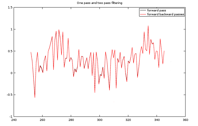
There are some hazards. The two-pass processing might not work at all for observer gains that are too far away from the Kalman optimum. Since the forward state transition step is presumed strictly stable, the reverse projection step is inherently unstable, and depends on the observer gains to keep things from coming apart. Be careful.

 

---