Linear Least Squares Review

In the previous installments, we reviewed the terminology:

• models
• linear models
• affine models
• independent variables (inputs)
• dependent variables (outputs)
• model parameter variables

We also considered the special case: the dynamic state transition models used by Kalman Filters.

We will now start thinking about practical tools for building these models — that is, for evaluating all of the numerical parameter values the model uses. For simplicity, we will start with simple input/output models — keeping in mind that these are not directly applicable to the purpose of Kalman filtering.

 

An example application

Lets suppose that the embedded application is required to monitor the temperature of a process. This temperature is supposed to be controlled to specified setpoint temperature within the range 50 to 90 degrees C. An effective way to measure temperatures in this range is with a "resistive thermal detector" (RTD) sensor device ^[1] . These sensors are ordinary resistors, but manufactured with selected pure materials and tight tolerances, to yield a resistance that varies in a highly linear fashion as a function of temperature. The most desirable material for this is platinum, which is stable and responsive over a wide temperature range. However, as you might expect, this is not exactly an inexpensive material. So, suppose that it is decided to manufacture an RTD device using a thin film of copper deposited directly on a circuit board. If the manufacturing process can be controlled well enough, and the thermal response can be modeled accurately enough, acceptable results are possible at low cost.

Let's assume that measurements of the resistance are good, unbiased, but not perfect; the measured values will show small random variations due to measurement error. Here is a table of the resistance vs. temperature data. The device is manufactured to have 10 ohms resistance, very closely, at nominal room temperature 25 degrees C, but as you can see, the resistance varies with temperature.

Temperature, deg. C	Resistance, ohms
0	9.04
5	9.23
10	9.42
15	9.65
20	9.81
25	10.00
30	10.19
35	10.39
40	10.58
45	10.77
50	10.97
55	11.16
60	11.35
65	11.58
70	11.74
75	11.93
80	12.12
85	12.32
90	12.51
95	12.70
100	12.90

 

Constructing the "linear least squares" problem

A linear sort of behavior is expected, except that the curve passes through 0 degrees C at a point where the resistance is not zero, hence the device model as represented in the table is not strictly linear. Propose a model in the following affine form, where values of model parameters a and b are to be determined, ti are temperatures, and ri are corresponding resistances as they appear in the table above. Variable i indexes the table rows.

$$t_i=r_i·a+b$$

The notation can be made simpler by collecting the terms into column vectors.

• column vector T contains the temperatures
• column vector R contains the corresponding resistance values
• column vector I contains the constant values 1.0 for every term

The tabulated data set can now be represented by the following vector notation. Each unknown parameter is a scalar (unknown) coefficient value multiplying a corresponding column vector. All vector terms are known.

$$T=R·a+I·b$$

We can simplify further using matrix notations. Package the unknown parameter values a and b to form the two-element parameter vector p. Consolidate the column vectors R and I to form matrix M with two columns and lots of rows, all terms known. Now the notation looks like a familiar matrix equation.

$$T=M·p$$

Solving for the unknown vector p would determine a model. But this system of equations has an unusual tall and skinny shape. With so many equations to satisfy and only two adjustable parameters to work with, it is unlikely that all of the tabulated conditions can be matched exactly, hence this system of equations will have no solution. Plan on it.

 

Best fit approximation

Instead of seeking a perfect solution, and failing, another approach is to look for an imperfect solution that, by some criterion, is as good as possible. This approximate solution might satisfy few or none of the constraint equations exactly. The so-called least squares solution is an approximate solution that minimizes the sum of the squared values of differences between predictions of the model and actual data. ^[2]

 

The necessary conditions for the "best fit" reduce to the following:

$$M^{T}M·p=M^T·T$$

This is the famous Normal Equations. If the problem is correctly formulated, the matrix product MT M should produce a square, nonsingular matrix with the same number of rows and number of columns as the number of parameters in vector p. The vector produced on the right-hand side of the equation will have a compatible number of terms. You can obtain a direct expression for the best-fit parameter solution by inverting the MT·M matrix.

$$p={\left(M^{T}M\right)}^{-1}·M^T·T$$

There are always concerns about whether a matrix equation was properly formulated so that a solution exists, is unique, and can be calculated accurately. But for purposes of building models, if you have formulated your least squares problem well: you should not expect problems. You will always verify your results, of course!

 

Back to the example

Applying this to the RTD example problem, if you construct the T, R, I elements as described, you will obtain normal equations as follow.

$$\left[\begin{array}{c}2555.562230.360\\ 230.36021.000\end{array}\right]\left[\begin{array}{c}a\\ b\end{array}\right]=\left[\begin{array}{c}1.2260e4\\ 1.0500e3\end{array}\right]$$

and the solution is

$$\left[\begin{array}{c}a\\ b\end{array}\right]=\left[\begin{array}{c}25.993\\ -234.468\end{array}\right]$$

Plugging in these values for the parameters in the proposed model form, the model predictions of temperature t can be calculated for each value of resistance r given in the table, and then compared to the temperature value that it should yield in the ideal case. Here is a plot of the model predictions (in blue) superimposed on a plot of the original data pairs (in red).

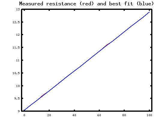
Where is the red curve, you ask? Look closely at the temperature range from 15 to 19 degrees C; also 63 to 69 degrees. You can just see a trace of the red curve. Everywhere else, the blue curve lands so closely on top of the red curve that the graphics cannot distinguish them. Not bad, huh?

But of course, this degree of success depends on fitting a linear model to something that really has a linear character. Having very clean and accurate data set also helps.

 

Quick review

We have reviewed the process of formulating a linear least squares problem.

• Collect the input data, the "independent variable data," into column vectors, with each column associated with one unknown parameter.
• If needed, supply an artificial "all ones" vector associated with a model parameter that is a constant to be estimated.
• Collect the desired output data, the "dependent variable data," into another vector.
• Set up the overdetermined matrix equation system, with the independent data matrix and unknown parameters on one side, the dependent output vector on the other.
• Reduce to the normal equations.
• Solve to determine the least squares best-fit model parameters.
• Insert the estimated parameter values in the model and apply to the original data, to evaluate the degree of success.

The matrix manipulations, though straightforward, can still involve some unpleasant grinding. The next installment will show how numerical tools can remove the drudgery from the calculations.

 

---