Least Squares Dynamic Fit

The strategy

Previous installments outlined the challenge, summarizing the features needed in a dynamic discrete model suitable for Kalman Filters, and describing the process of formulating a Linear Least Squares problem that can be solved to estimate model parameters.

Let's now make a bold attempt to put some pieces together, and derive a dynamic model having an appropriate form from numerical input/output data. As far as model quality — well, that will have to wait until later.

 

The system

I could know how the system input output data was obtained; but I choose not to. Ordinarily, it is not a matter of choice. I have no idea how a model fit might turn out. Since models are not unique, there are lots of possibilities.

There is one system output variable, and there is one system input variable. The behavior is somewhat complicated, so the system order is presumed to be around 5. Let's try that and see what happens. Too low, and there will probably be some serious accuracy problems; too high, and there will probably be some redundancy and possibly some numerical problems.

We know that the system output predicted for the next output instant will depend on the current system state, and also on the current inputs.

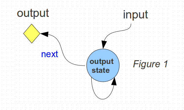
Tracing this back one step in time, there is the possibility of another state that influences the value of the first state, but otherwise, its effects are not visible in the outputs until they propagate into the first state.

In this same manner, there can be more hidden states that take even longer to directly influence the outputs.

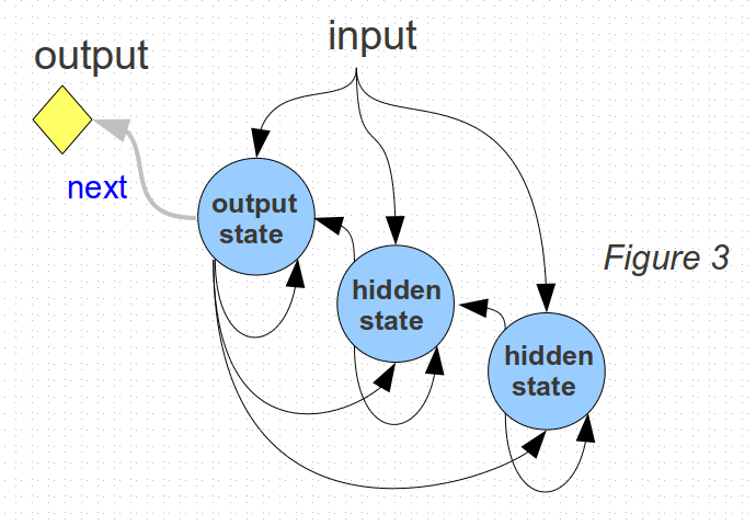
Under the presumption of a fifth order model, this can continue until there are up to 5 states.

The problem is: the state variables are internal and invisible. Since up to 5 time steps are needed to be sure that all of the presumed states have a chance to influence the output values, I will preserve 5 collected values of the inputs and outputs for fitting the model.

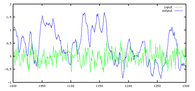
Here is how a typical run of system input and output data appears.

That accounts for "the current data", but what about the "past history?" When there is a long sequence, the "past history" vector looks just like the "current data" vector — except that the entire column data is shifted one position. Past history two steps back would be a data vector shifted two positions, and so forth.

vectors of current and past output values
  current:    one step past:  two steps past:
    1.26          1.21           1.16
    1.32          1.26           1.21
    1.38          1.32           1.26
    1.45          1.38           1.32
    1.52          1.45           1.38
    ...           ...           ...

The independent variable values for the model fit are therefore 5 columns of current and past output values, along with 5 more columns of current and past input values.

Using the superscript notation to express the position in time — or equivalently, the amount that the data column is shifted — we would like the linear model to represent the following observed input/output relationships, where the a and b terms are the model parameters to be determined.

  yN+1 = b0·yN+0 + b-1·yN-1 + b-2·yN-2 + b-3·yN-3 + b-4·yN-4 
       + a0·uN+0 + a-1·uN-1 + a-2·uN-2 + a-3·uN-3 + a-4·uN-4

Taking N = 5, 6, 7, etc. through a very large number of terms (let's use 10000) we can construct a vector for each term, and then express the target conditions in the form of a matrix equation.

 
  yN+1 = [yN+0   yN-1   yN-2   yN-3   yN-4   uN+0   uN-1   uN-2   uN-3   uN-4   ] ·
        [ b0    b-1    b-2    b-3    b-4    a0    a-1    a-2    a-3    a-4 ]T

The matrix of a and b terms has the model parameters to be determined. That extra transpose operation is, of course, just a reminder that the parameter terms must form a column matrix to be compatible with the matrix multiply operation in the model.

There are two data matrices. The first, consisting of independent variable vectors with lots of terms, is very tall and narrow. The column vector of output terms will have the same large number of rows. This is typical of Least Squares fitting. We will try this 10000 rows... probably not enough, but we have low expectations and want to start easy.

This equation system is vastly overdetermined. We can use Linear Least Squares methods to obtain an approximate solution. You know exactly how to do that from the previous installment. So at this point, let's skip ahead to the numerical result.

 

The solution

Here is the model fit that results.

  -0.3757921       Parameters for input history
  -0.1939514
  -0.0527318
   0.0051917
   0.0230597
   0.9000531       Parameters for output history
   0.0698574
   0.0249757
  -0.0734740
   0.0148904

And as always, we will check how well the fit compares to the actual data.

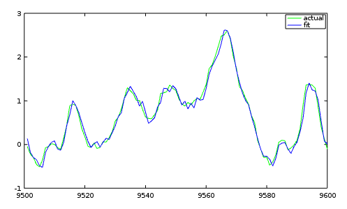
For such an unsophisticated analysis, we have a rather better fit than we might have expected. We must be very close to a solution. Or are we? We overlooked something of major importance, and we need to take a closer look next time.

 

---