Introduction
Other sites:
Hamming [1] suggested the way.
Spoiler alert: you can design derivative estimator filters with pretty much any degree of accuracy you want, and with whatever high frequency noise rejection you want, but you must either be prepared to invest some effort to achieve it, or grab a pre-built reference design as "good enough." Though theoretical performance is outstanding compared to other designs, filter evaluation takes at least twice as much computation as other designs.
Properties of a Derivative Operator
A derivative operator will take a cosine wave, which is real symmetric, and produce from it a negative sinewave of the same frequency — real and anti-symmetric. We know that an anti-symmetric real sequence will have a Fourier spectrum with zero real-valued parts. Examining the derivative of a cosine wave, as the normalized frequency in the sampled data varies from 0 to 0.5 of the normalized sampling frequency (2 samples per waveform cycle), we find that the magnitude of the derivative signal runs from 0.0 to -π. This means that in a Discrete Fourier Transform (or FFT) the imaginary terms in the first half of the transform block will range from 0.0 to -π while the real terms are zero.
From symmetry properties, we know that the second half of an FFT (nominally, for frequencies from 0.5 to 1.0 of the normalized sampling rate) is the complex conjugate of the first half of the spectrum. So, the transform is completed by filling in the numbers from +π to zero.
This completely defines the frequency domain response of a theoretically ideal differentiator. In concept, this can be converted back to a time domain operator by calculating the inverse FFT. However, this would have all the undesirable high-frequency noise response properties of other designs. As we know, we only want the derivative estimator to match the ideal curve through a limited range, otherwise high frequency noise will dominate the results.
Extending R. W. Hamming's scheme
A practical design should accurately track the ideal differentiator frequency response curve up to about normalized frequency 0.1. Above that, the frequency response should begin to roll off. Above frequency 0.25 or so, the filter response should be close to zero. At normalized frequency 0.50, the Nyquist Limit is reached, and there is no no unambiguous interpretation of the data beyond this point.
The scheme that Hamming suggested was as follows.
-
Over some range that you want to approximate, set the spectrum terms to the desired ideal response line.
-
Everywhere else in the spectrum, specify that the values should be zero.
-
Take the inverse transform of this spectrum.
-
Apply a suitable window to truncate the filter to a desired number of terms.
There was a reason for using this approach: the theory is easy. But if the truncation results in discarding terms of any significance, the resulting filter can produced persistent "Gibb's phenomenon" oscillations. Rather than truncating a spectrum curve, another option is to select a suitable smooth "windowing" curve that attenuates the values gradually instead of cutting them off sharply. There is a slight loss of accuracy, particularly for higher frequencies, but there is a net benefit of producing a shorter filter with acceptable results.
I chose to pre-shape the filter response spectrum so that it had exactly the right values at low frequencies, exactly zero at high frequencies, and a smooth transition between these regions. More specifically, the sequence of multipliers to shape the spectrum has the following properties:
- the curve is continuous in value
- the curve is continuous in derivative
- the curve tracks the desired band exactly
- the transitions go smoothly from the ideal curve to zero
- the curve equals zero for higher frequencies
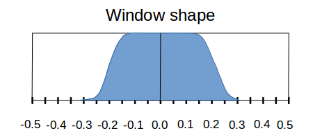
I chose for the frequency window a flat "plateau" (similar to a rectangular window), centered on zero frequency, with smooth "tails" similar to a von Hann window dropping down to zero at the high frequencies.
Obtaining the filter terms
Use an inverse FFT to convert the shaped spectrum into filter coefficients in a time sequence. By construction, the FFT result is an anti-symmetric real sequence. Discard any imaginary parts, because they consist of nothing more than numerical roundoff noise.
The high-frequency terms are very small, but not exactly zero. Keeping all of these tiny terms in the filter is inefficient. One approach is to simply force all of the very small terms to exactly zero. However, this is another kind of "abrupt truncation" that tends to have unintended consequence. A conventional technique to suppress the small terms is to apply a finite-length window to the filter coefficients, multiplying the window term-for-term with the raw transform result. The length of the window vector dictates how many terms remain in the final filter.
Hamming recommended using a Kaiser window for this final windowing operation. It is close to optimal for most purposes, and it has an adjustable window-width parameter, which allows a tradeoff between the narrowness of the transition shape and the high-frequency ripple rejection. I took his advice on this; it worked out very well.
To recap, these are the adjustable parameters used to obtain the filter design:
-
For the frequency domain, the number of terms in the "flat plateau region" of the spectrum-shaping window. In concept, this defines the band that you want to attempt to match exactly. In practice, this approximately positions the peak of your filter response. When windowing is applied later, terms before and after this point will be affected, so leave extra terms in the "accurate region" to allow for this. For example, a range
170was selected, meaning 170 locations out of a 1000 point FFT were specified for the accurate band. I actually only wanted accuracy through 0.10, so the extra terms from 0.10 to 0.17 anticipate curvature effects of windowing. -
The number of terms in the "cosine transition shape" of the frequency domain spectrum shape. The wider this is, the better the tracking accuracy in the band you want, but the more noise enters through the transition band frequencies. For example, I selected a the transition size
84. The spectrum curve then drops to 0 after location 170+84 (normalized frequency 0.254) in a 1000 point FFT. -
The number of terms you wish to preserve in the final filter, which is also the number of terms in the final Kaiser "clean-up" window. For example, I set the Kaiser window to have 25 terms, in order to obtain a 25 term final filter length. You can use more terms to incrementally improve the noise rejection at the expense of more computation when the filter is applied.
-
The windowing parameter of the Kaiser window. The larger this parameter is, the greater the ripple suppression at the expense of a wider transition shape. Typical parameter values are 3.5 to 7. For example, I used the parameter value 6.2, because a 25-term filter is becoming small and aggressive ripple reduction is needed.
To build the filter according to these parameters, enter them into the filter design script. This script implements all of the steps previously described. Let it grind out the coefficients.
This script also uses
a separate window construction function
that you will need. Download these script files and change the file
extension from -mfile.txt" to .m. The
design script is intended to be
compatible with GNU Octave / Mathworks Matlab. These scripts are submitted to
the public domain, hence free as in beer, and also free as in
freedom, but it does not mean free as in no worries. If you
choose to use this, you are strictly on your own. You have been warned!
Here is the results of a design using the parameter values given as examples above:
match = 170; transit = 84; nfilt = 25; alpha = 6.2;
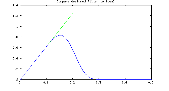
 % High-performance derivative estimator
filter1 = [ ...
  -0.000128291316161,   -0.000421427471795,    0.001039598292226, ...
   0.003793406986458,   -0.001298001343678,   -0.015244969850269, ...
  -0.008439774762739,    0.036664149706911,    0.052652912201092, ...
  -0.049494997825050,   -0.204043104762539,   -0.207564884934383, ...
   0.000000000000000,    0.207564884934383,    0.204043104762539, ...
   0.049494997825050,   -0.052652912201092,   -0.036664149706911, ...
   0.008439774762739,    0.015244969850269,    0.001298001343678, ...
  -0.003793406986458,   -0.001039598292226,    0.000421427471795, ...
   0.000128291316161  ] ;
This design matches the ideal curve from frequency 0.0 to frequency 0.10 within a 0.01% error. The noise rejection outperforms all of the other formulas I have found so far.
Conclusion
If you need accuracy and noise insensitivity, the FFT-based differentiator filter designs can give you excellent accuracy through the frequency range you need, with excellent noise rejection, but producing a design can require a lot of effort. Because the filter has quite a lot of terms, evaluation requires extra computation, but that is part of the compromise. Many applications can just grab the "example design" as given above and go with that. It spans a block of 25 data samples.
While the filter length might seem rather excessive compared to other designs, perhaps this is not as bad as it first seems. Suppose that your approach to the problem is to first apply a well-selected lowpass filter to the data, to remove undesirable high frequencies; then apply a simple differentiator formula like Central Differences. Between the smoothing and the differentiator filters, this might involve more numerical effort than the FFT-based estimator in a single pass.
Though performing well, there is something troubling about the large amount of computation. Perhaps an overkill amount of numerical effort is directed toward forcing all of the high-frequency noise exactly to zero. I speculate that a truly optimal design would show some kind of bounded but not monotonic noise rejection properties, with zero crossings at high frequencies in the manner of the "Alternation Theorem." [3]
Footnotes:
[1] Digital Filters, R. W. Hamming.
[2] Experiments with the much simpler least-squares designs were described briefly elsewhere on this site.
[3] For background on Chevyshev equal-ripple approximations, try
http://en.wikipedia.org/wiki/Approximation_error.