PID vs. State-Space Linear Control — Really?

Which one is better?

I have seen the arguments.

• State-space models produce superior results.
• PID is ready off the shelf and works well enough, so why mess around?

If you don't have a model for how your system works, you might not have much choice. In such circumstances, you won't be able to do much more than apply heuristic controls. The heuristics for PID control are as follows:

1. The proportional correction rule. The more the system output deviates from the level you want, the harder you should try to correct it.
2. The integral correction rule. If the output level remains persistently displaced, adjust the control output level cumulatively to correct for this.
3. The derivative correction rule. If the output is changing too fast, reduce the control output to avoid speeding past the desired output level.

The three rules propose different output strategies. The conflict is resolved by taking a weighted sum of the recommendations from the three rules.

While steeped in plausibility, there are all sorts of subtle ways that this control scheme can perform poorly: taking too long to reach the desired setpoint level, applying excessive corrections that rattle the system, bouncing around in low level oscillations, and so forth. Even when the control is successful, selecting gain settings to give best results remains more alchemy than science.

Simulation using a mathematical model is a valuable technique for understanding what is happening in a system. When you have a model that reflects the actual behavior of your system, and a control strategy that works well for your model, that control strategy has better chance of working on the real system than one based on plausibility alone. One type of model that works very well for a lot of systems is a state-space model, in which a set of state variables (such as temperatures, pressures, fluid levels, speed, and so forth) characterize what the system is doing; a set of differential equations then describes how input variables interact to change the system state. An important special case of a state-space model is a linear state-space model , in which the input/output and differential equation systems are linear. This is not strictly realistic, but it works well enough and often enough that it is the only case considered here. (Of course, the ideas can be extended to a nonlinear case if you insist!)

Suppose you have developed a model, and determined a typical linear feedback rule that shows good control results. Now you want to implement your strategy on the real system. Good luck with that. When you go shopping for equipment to apply your ideas, you will find that PID controllers are available, but precious little else. In the end, all of your efforts to model and understand the system get thrown out the window.

Maybe it doesn't have to be that way. General linear feedback schemes based on a state space model can use multiple observed variables to produce multiple control output signals. PID schemes are linear and use one observed system variable to produce one control output. It would seem like the PID case should be easier. What prevents it from being incorporated into your state-space model?

Check out the following. I have never seen an analysis of this sort in print elsewhere. It may be old business. If this is the case I apologize in advance.

 

Augmenting the System Model

Assume that you have a linear state space system model of your system, with state vector x, a single-variable control v applied through system input u, continuous state matrix a, input coupling matrix b, and observation matrix c to observe the relevant system output y. Though, in general, the y vector can provide several observed variables, for now, we consider only the one output of relevance to the PID control.

System Model

$$x\prime =ax+bu$$ $$y=cx$$

We will consider the input u to consist of two parts: a setpoint driving term s, and a feedback term v, with separate input coupling matrices bf for the feedback, and bs for the setpoint. (For purposes of simulation, a third input variable with coupling matrix can be included to represent a class of disturbances.) The separation will make it a little easier to think about the setpoint and feedback signals individually.

Looking ahead, we know that PID control rule will need to compute the differences between the observed output variable and the setpoint. The setpoint will need to be an additional observable quantity. For now, the tracking error e = y−s, is treated as a separate observed variable, and the notation will be consolidated later.

Reorganized system model

$$x\prime =ax+b_{f}v+b_{s}s$$ $$y=cx+0s$$

$$e=cx+-1s$$

A PID controller (in parallel form) applies three control rules to perform the its computations. Each of these rules observes variables dependent on setpoint and system state.

 

proportional control

Proportional feedback responds in proportion to the difference between the desired output (setpoint) and the observed system output. The current value of the tracking error e is needed. The proportional feedback rule is:

proportional feedback rule

$$v=-k_p\left(y-s\right)=-k_{p}e$$

The scaling factor kp is the proportional gain of the PID controller.

 

integral control

To detect a persistent tracking error, the PID controller integrates the tracking error e over time. Augment the system equations with an additional artificial state variable z to represent the state of the accumulator. Include this as an extra row in the state equations. The integration that solves for other state variables then updates the error integral term at the same time. Since the tracking error integral value is needed for feedback calculations, the observation equations must be augmented to present the value of variable z.

integral feedback rule

$$z\prime =e$$ $$v=-k_{i}z$$

The scaling factor ki is the integral gain of the PID controller.

 

derivative control

The derivative part of a PID controller is somewhat fictional. A real PID controller observes changes in its signals and from this estimates what the derivative must be. If you know exactly how it produces this estimate, you could include that same calculation in your model. Most likely, you don't know, so you must provide something based on your state-space model.

Derivatives for any output value can be obtained by substituting the derivative relationships in the state update equations into the output observation equation. The variable you should use is the derivative of the system output variable. This is not the same exact thing as the derivative of the tracking error, as defined in classical PID control — but actually, this is better, because the derivative of the tracking error and the derivative of the output variable will be the same except at instants where the setpoint level changes. And at those points of discontinuity, the tracking error derivative is undefined. (PID controllers are famous for giving the system a severe jolt through the derivative feedback term when the setpoint changes. Unnecessary and avoidable!)

The derivative estimate produced by actual PID equipment remains sensitive to high frequency noise. High frequency means rapid change, which means large derivative. On the presumption that extreme high frequencies are not a natural part of the system response, lowpass filtering is often applied to limit the bandwidth of the derivative estimate. While this is typically beneficial, it can also introduce new hazards. If you know what the filtering is, you can include that calculation exactly in your model.

Keeping in mind these considerations, the derivative of the output variable as predicted by the state equations is:

derivative control rule

$$y=cx$$ $$y\prime =cx\prime =cax+c{b}_{f}v+c{b}_{s}s$$ $$v=-k_{d}y\prime =-k_{d}c\left(ax+b_{f}v+b_{s}s\right)$$

where kd is the derivative gain of the PID controller. This expression presents a problem: the feedback variable v appears on both sides of this expression. An algebraic reduction can combine the two v terms. Define the algebraic factor Kg, and use it to simplify the derivative feedback expression above.

derivative feedback after algebraic reduction

$$K_g=1/\left(1+k_{d}c{b}_f\right)$$ $$v=-k_d{K}_{g}c\left(ax+b_{s}s\right)$$

For many and possibly most systems, the feedback v does not couple directly and instantaneously into the output variable y — and for this common case the c bf product evaluates to zero. The Kg term then reduces to a value of 1 and can be ignored.

 

Consolidating the Augmented State Model

To integrate the feedback calculations with the rest of the model, start by collecting the additional observed terms that were mentioned in passing. These are appended to the original y vector.

original output variable

$$y=cx$$

 

supplemental tracking error variable

$$y_p=z=cx-s$$

 

supplemental integral-error variable

$$y_i=z$$

 

supplemental output derivative calculations

$$y_d=K_{g}c\left(ax+b_{s}s\right)$$

 

augmented observation vector

$$Y=\left[\begin{array}{c}y\\ y_p\\ y_i\\ y_d\end{array}\right]$$

The augmented state includes the supplemental integral-error variable. The PID calculations use this additional state information, but for all other purposes, the artificial state variable is ignored. The input coupling matrix gets an additional row for driving the new tracking error integral, but of course the new row be in this matrix will consist of a single term equal to 1, applied to the tracking error term, with all other coefficients equal to zero.

augmented state with tracking error integration

$$X=\left[\begin{array}{c}x\\ z\end{array}\right]$$

input vector with feedback and setpoint terms separated

$$U=\left[\begin{array}{c}v\\ s\end{array}\right]$$

augmented input coupling matrix with error integration row

$$B=\left[\begin{array}{c}{b}_f{b}_s\\ b_{e}0\end{array}\right]$$

augmented state matrix with tracking-error integration

$$A=\left[\begin{array}{c}a0\\ 00\end{array}\right]$$

augmented state equations

$$X=AX+BU$$

Now the coefficients appearing in the augmented observation equation can be reorganized into a matrix form that provides the extended list of output terms, with one column applied to the original state, and the second column using the new tracking integral, making it visible for the PID calculations. A new input coupling matrix D is added for the purpose of making the setpoint value available to the tracking error calculation and the derivative estimate.

augmented observation matrix

$$C=\left[\begin{array}{c}c0\\ c0\\ 01\\ K_{g}ca0\end{array}\right]$$

augmented observation input coupling matrix

$$D=\left[\begin{array}{c}00\\ 0-1\\ 00\\ 0K_{g}c{b}_s\end{array}\right]$$

augmented observation equations

$$Y=CX+DU$$

 

Calculating the PID Feedback

Thanks to the way that the observation vector has been defined, the PID feedback can be represented as a linear feedback in the typical manner for linear state-space models. The original output variable, y, is not used directly. The first row in the feedback vector contains the collection of PID gains. The second row is a trivial one that merely reports the value of the current tracking error for purposes of updating the error integral.

PID feedback gain matrix

$$K=\left[\begin{array}{c}0k_p{k}_i{k}_d\\ 0100\end{array}\right]$$

feedback control law

$$v=-KY$$

 

We have just obtained a state-space model with linear feedback for a system under PID control. This is a matter of notation, not control theory. Because it is clear that this represents a PID control, and that it is a state-space representation, there is no theoretical need to choose between PID or linear state-space control theory for purposes of system analysis. That choice might be need to be made because of other practical restrictions, such as the opportunity or difficulty for developing the necessary system model.

 

An Example

A hypothetical system is constructed deliberately to be extremely difficult for a PID controller, so that the simulation always has something to show regardless of the gain settings. The problem is to cancel out observed displacements in one of the variables, by controlling an input that drives another variable. The two variables change out of phase, consequently the PID controller might need "negative feedback gains" of the sort that would drive ordinary systems straight to instability.

The desired disturbance level is 0, so the setpoint variable s is 0 and the bs terms are otherwise unused. For this simulation, the spare bs vector is used artificially to insert a simulated disturbance.

Here is the original system model, with the third state variable observed for feedback, while inputs drive the fourth state variable.

sysF = ...
[ 0.0     0.0     1.0    0.0; ...
  0.0     0.0     0.0    1.0; ...
  -0.052  0.047  -0.01   0.0; ...
  0.047  -0.052   0.0   -0.04 ];

sysB = [ 0.0;  0.0;  0.0;  0.01 ];

obsC = [ 0.0;  0.0;  1.0;  0.0 ];

There is a PID controller, separately modeled, with gains

kp = 2.0; ki = -.50; kd = -15.0;

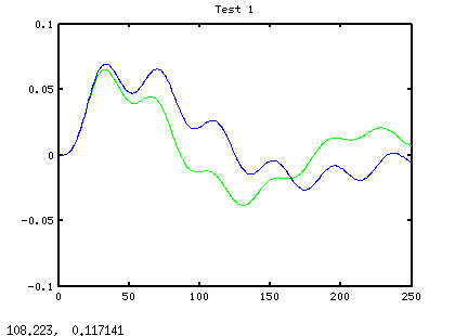
This is simulated with time-step delT = 0.5 through 250 steps, using a trapezoidal rule integration for the system state model and rectangular rule integration for the PID integral term. The following plot shows the state 3 that we would like to regulate to 0. The green trace is without feedback control, and the blue trace is using PID control.

So now the problem is reformulated to include the PID controller within the state space model. Because the feedback drives one variable, but output sees a different variable, there is no direct coupling into the derivative term. The Kg term reduces to 1.0 and can be omitted. Here are the augmented equations:

sVar = 1.0;
setpt = 0.0;

sysF = [ ...
  0.0     0.0     1.0    0.0   0.0; ...
  0.0     0.0     0.0    1.0   0.0; ...
  -0.052  0.047  -0.01   0.0   0.0; ...
  0.047  -0.052   0.0   -0.04  0.0; ...
  0.0     0.0     1.0    0.0   0.0 ];

sysBset = [ 0.0;  0.0;  0.0;  0.01;  1.0];

sysBfb  = [ 0.0;  0.0;  0.0;  0.01;  0.0];

obsC = [ ...
  0.0     0.0     1.0    0.0   0.0;  ...
  0.0     0.0     0.0    0.0   1.0;  ...
  -0.052  0.047  -0.01   0.0   0.0;  ...
  0.0     0.0     1.0    0.0   0.0 ];

obsD = [ -1.0;  0.0;  0.0;  0.0 ];

pidK = [ 2.0  -0.50   -15.0   0.0 ];

Here is the simulation for the augmented system, recording the state trajectory for later inspection.

sVar = 0;
for i=2:steps
  % Current state and observed variables
  xstate = hist(:,i-1);
  yobs = obsC * xstate + obsD * sVar;

  % Feedback law applied to current output
  fb(i) = -pidK * yobs;

  % Predictor step (Rectangular rule)
  deriv = sysF * xstate + sysBset * sVar + sysBfb * fb(i);
  xproj = xstate + deriv*delT;
  yobs = obsC * xproj + obsD * sVar;

  % Corrector step (Trapezoid rule)
  dproj = sysF * xproj + sysBset * sVar + sysBfb * fb(i);
  xstate = xstate + 0.5*(deriv+dproj)*delT;
  hist(:,i) = xstate;
end

Here is the result of this simulation.

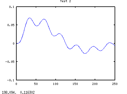
At first glance, it is a match for the previous simulation. It has captured the essential behaviors of the PID-controlled system. However, the results of the two simulations do not really match exactly, and we should not expect them to, because a state-space model calculates derivatives, while an ordinary PID controller estimates them.

---