Motivation
I was not successful in producing good results with the Voss- McCartney algorithm as described by Allan Herriman and listed in the "DSP generation of Pink (1/f) Noise" web article at http://www.firstpr.com.au/dsp/pink-noise/.
Here was the problem. As indicated by the text-art illustrations on that site, each component stage in the Voss-McCartney generator produces a sequence of randomly modulated squared pulses. For pulses produced at a given frequency, they produce spectral energy distributed according to the familiar/accursed sin(x)/x form. That is, the spectral energy distribution is NOT SMOOTH. Certain frequencies are supplied plenty of energy, and certain others get zero. The following plot shows the power spectrum of a single simulated stage. Please note, this is not a plot of theoretical formulas, it is from numerical operation of the generator and lots of averaging.
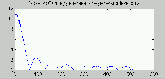
When multiple generator stages of the Voss-McCartney generator are combined, each one contributes energy in the same non-smooth manner, with each one compressed more toward the low-frequency end of the spectrum, making it less able to compensate for anomalies produced by the higher frequency updates. The combination depends on the harmonic frequencies, and it is not random. If the peaks of one power distribution happen to line up well with the valleys of previous ones to compensate, the combination could well approximate the 1/f power characteristic. But otherwise...
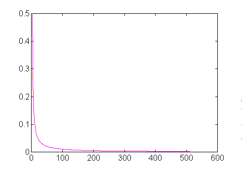
I experimented with this empirically, simulating the generator and using FFT methods to analyze 10000 replications of 1024-term sample blocks. The power distribution characteristic was starting to show the desired 1/f form, but it was clear that a very large number of stages would be needed to have any chance of an accurate approximation. For example with eight stages, compare actual results to the ideal 1/f model:
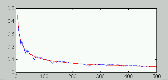
It was pretty clear that this was not converging uniformly and rapidly to an accurate fit.
Why This Result?
It seemed to me that the reason for the non-smooth spectrum curves was the fact that the updates are highly predictable. If a low frequency generator is updated, there are only certain discrete times at which this will happen. It is this high degree of non-randomness, so I conjectured, that causes the repeatably irregular spectrum shape.
My idea was this: would the generator performance be better if the
generators were updated at the same rates ON THE AVERAGE, but not on a
rigid schedule? That is, the times at which updates occur are
randomized to occur with probability p
for the first stage, probability p/2 for the second, ...
probability p/2N for stage N.
With this scheme, each generator is updated the same as the Voss-
McCartney generators on the average.
In the following experiment, I picked a single stage and updated it repeatedly. I then did an FFT analysis, scaled the result, and obtained the following comparison to the ideal 1/f spectrum (I believe this is a magnitude rather than power spectrum)
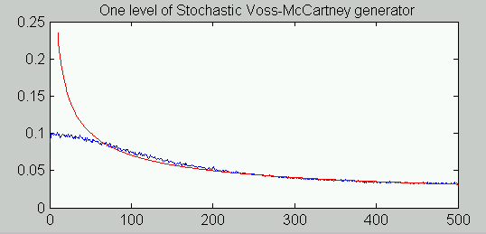
This was an encouraging degree of similarity.
Expanding the Randomized Generator Experiment
I tried adding more stages, but I was disappointed with the results. The range was extended downward as expected, but the tracking of the 1/f shape was not accurate.
I suspected that this was related to the aliasing phenomenon
in sampled data systems, with higher frequencies reflecting
in the sampled data set as distortions of the desired curves leading
to a flattening of the spectrum. Wishing to avoid an exact
analysis at this point, I wondered whether a different scaling
on the generator terms would produce a more accurate fit. Here is
the Stochastic Voss-McCartney Algorithm after generalizing the
stage weighting parameters. The urand function is a uniform
pseudo-random generator on balanced interval -1 to 1, obtainable
from generators on interval 0 to 1 by the mapping
2*(rand-0.5).
  Weighted Stochastic Voss-McCartney Algorithm (first version)

  For each update:
    level  := urand[0,1]

    output := urand[-1,1]*W1
    if (level>0.5) break;
      output := output + urand[-1,1]*W2
    if (level>0.25) break;
      output := output + urand[-1,1]*W3
    if (level>0.125) break;
      output := output + urand[-1,1]*W4
    if (level>0.0625) break;
      output := output + urand[-1,1]*W5
    if (level>0.03125) break;
      output := output + urand[-1,1]*W6
    if (level>0.015625) break;
      output := output + urand[-1,1]*W7
    if (level>0.0078125) break;
      output := output + urand[-1,1]*W8
    if (level>0.00390625) break;
      output := output + urand[-1,1]*W9
  End
I experimented with another variation that generated the
level decision random variable for each test
independently and this didn't make any difference. For my first tests,
the scaling parameters W1 through W9 were
initially set equal, as in the original Voss-McCartney algorithm, and
then I began tweaking manually to see where this would lead. I ended
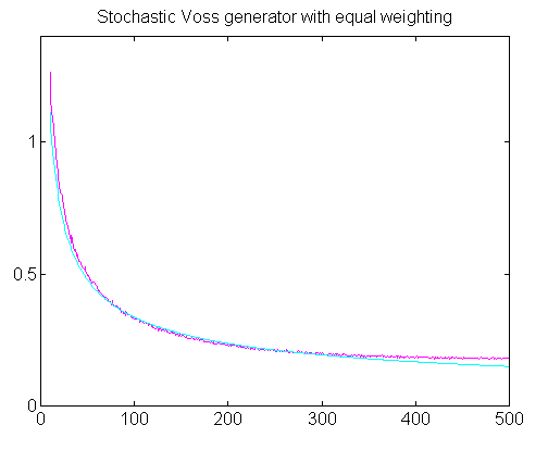
up with the weighting factors
Weighting factors: W1 - W9
    .252
    .672
    .000
    .171
    .190
    .286
    .175
    .233
    .021
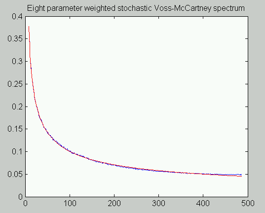
The attached illustration shows simulated results of the 8-stage random generator with adjusted weights. Don't get too excited about this, because we can do better.
An Additional Generalization
The spectrum has the shape it does because of correlation between terms in the composite generator. In the analog world, the 1/2, 1/4, 1/8 sequence for probability of updating should produce the right shape, but that is an infinite sequence and it breaks down in sampled data systems. As a second generalization of the original algorithm, I considered allowing adjustment of the correlation by adjusting the probability levels for updating at each stage. This yielded the (final?) Stochastic Voss-McCartney Algorithm.
  Weighted Stochastic Voss-McCartney Algorithm

  For each update:
    level  := urand[0,1]

    output := urand[-1,1]*W1
    if (level>L1) break;
      output := output + urand[-1,1]*W2
    if (level>L2) break;
      output := output + urand[-1,1]*W3
    if (level>L3) break;
      output := output + urand[-1,1]*W4
    if (level>L4) break;
      output := output + urand[-1,1]*W5
    if (level>L5) break;
      output := output + urand[-1,1]*W6
    if (level>L6) break;
      output := output + urand[-1,1]*W7
    if (level>L7) break;
      output := output + urand[-1,1]*W8
    if (level>L8) break;
      output := output + urand[-1,1]*W9
  End
This adds no new complexity to the code, but it does add
another degree of difficulty to the analysis. How do you pick the
right correlation parameters L, and how good of a fit is possible?
It was time to do the homework. Along the way, I found an
alternative scheme for the individual generator stages.
Correlated Generators
Generator Type 1
Consider the following stochastic processes, based on the randomized version of the Voss-McCartney generator stages.
    Rk =
    |  Rk-1 with probability p
    |  r distributed U(-1,1) with probability (1-p)
The random variable r is an uncorrelated random
number as approximated by a uniform random number generator algorithm.
With each sample the value of generator R either remains
the same, with perfect correlation, or it is allowed to change
to a new value completely independent of all past history. The
less often a generator's value changes, the more its output
looks like a low frequency pulsed wave, and the more the
generator stage contributes its signal energy at low frequencies.
Properties of the distribution of r:
    E(r) = 0            (zero mean)
    E(r2) =  1/3         (variance)
From these properties of r we can immediately deduce
the expected value
E(Rk·Rk) = 1/3
Considering a one step delay, the autocorrelation at this interval depends on
    Rk · Rk =
    |  R2k-1   with probability p
    |  Rk-1 r   with probability (1-p)
But from independence, the expected value of the second product pair will be zero, so we will obtain
E( Rk · Rk-1 ) = p/3
Continuing in a similar manner by induction, and observing that the correlation function is symmetric, we obtain in general
E( Rk · Rk-N ) = p|N|/3
In other words, the correlation sequence is exponential. But there is another way to generate the exponential correlation in a random sequence, which I already knew about, and this leads to another form of generator stage that can be used with equivalent effect.
Generator Type 2
Consider the alternative generator form that is updated at every sample but with a partial replacement, adjusted by a parameter p in the open interval (0,1).
Rk = Rk-1·p + r·(1-p)
The algebraic derivation is omitted, but it can be demonstrated that
E( Rk · Rk ) = (1-p) / 3(1+p)
and from there that
E( Rk · Rk-N ) = (1-p) / 3(1+p) · p|N|
That is to say, the correlation is once again exponential, and
differs only by a scaling factor depending on parameter
p, hence the adjustment to make the two generators work
equivalently for the pink noise generation is a simple scaling.
The second generator form is just the discrete time equivalent
of a linear first-order lag filter. Increasing p and
increasing the correlation is closely related to increasing the
"lag time constant" in a linear first-order lag, which means that
larger values of p result in a lower cutoff frequency.
Possible advantages from this second correlated generator
form: the power distribution might show a little less variance over
the short run, and the computational load is uniform for every
update. I also speculate that higher order statistics would
correspond better to a true pink noise process. The amplitude
coefficients I provide later do not take into account the additional
scaling factor, so you would need to adjust by (1+p)/(1-p)
when applying the second generator form.
For completeness, the following is the stochastic correlated generator algorithm using the second type of generator stage.
  Correlated Generator Algorithm

  state[1:Nstages] = 0.0;
  for each update:
    output = 0;
    for iSt = 1:Nstages
      state[iSt] = P[iSt]*state[iSt] + (1-P[iSt])*urand(-1,1)
      output = output + Wt[iSt]*state[iSt]
    end
  end
Power Spectrum Analysis
After an unbelievable length of time messing around with approaches that were nonproductive, I settled down to basic z- transform theory and found the mathematical model that exactly describes the power spectral density contributed by each individual generator stage. The combined power of the independent sources is then the sum of the spectral power from each generator.
Start with the autocorrelation function for the generator, ignoring the extra scaling factor that will be present for the type-2 correlated generator stage.
E( Rk · Rk-N ) = p|N|/3
Applying the definition of a z transform and splitting the infinite sum into a positive one-sided transform, negative one-sided transform, and constant term, we get the power spectrum
   S(z) = sum( Rn z-n )   over all n

        = 1/3 · 1/(1-pz-1)  +  1/3 · 1/(1-pz)  -  1/3
An algebraic reduction yields the equivlent formulation
       1/3 · (1-p2) z-1
     ---------------------------
       (1+p2)·z-1 - p·(1+z-2)
For purposes of evaluating the power spectrum, we can ignore the
z-term multiplier in the numerator as this is just a time
shift, which doesn't matter. Otherwise, we can make the usual substitution
z = ej·2·pi·n/N
where N is the number of frequencies to sample between 0 and the sampling rate, and n is the frequency term index. However, due to the special symmetry in this expression, the remaining imaginary terms cancel, and we end up with a simple analytical form.
            1/3 · (1-p2)
   S(n) = -----------------------
           (1+p2) - 2p·cos(An)
where angle step A equals 2·pi/N.
The relevance of this is that we now have a relatively simple and very precise numerical formula that says exactly how much signal energy each generator stage is going to introduce at every frequency, as a function of correlation adjustment parameter p. Thus, we have all of the information necessary to numerically optimize both the generator probability parameters and the generator scaling factors, for any given number of generator stages M.
Optimizing the Generator Parameters
There is no hurry in doing this, as the problem is small scale, and I used a slow, steady, reliable — did I mention slow? — gradient algorithm to tune the coefficient settings. Unfortunately, the dependence on the p parameter is nonlinear, so a nonlinear optimization is necessary.
I used Matlab code to perform this optimization and display the results, and I can make it available to anybody who wishes to pursue this further, with the understanding that it comes with no warranty and you are on your own to correct the errors and make it work right. For most people, the following parameter sets should cover most requirements. These seem to take the stochastic generator algorithm very close to the absolute limits of what it can do.
| Number of terms |
Band covered | Fit error | Coefficients |
|---|---|---|---|
| 3 |
2.5% to 80% of Nyquist frequency (5 octaves) |
0.25 dB |
a = [ 0.01089 0.00899 0.01359 ] p = [ 0.3190 0.7756 0.9613 ] |
| 4 |
1.25% to 75% of Nyquist frequency (6 octaves) |
0.15 dB |
a = [ 0.01000 0.00763 0.00832 0.01036 ] p = [ 0.3030 0.7417 0.9168 0.9782 ] |
| 5 |
0.8% to 80% of Nyquist frequency ( 7 octaves ) |
0.15 dB |
a = [ 0.00224 0.00821 0.00798 0.00694 0.00992 ] p = [ 0.15571 0.30194 0.74115 0.93003 0.98035 ] |
Here is a listing of Matlab code extracted from my test scripts. It is configured for a three-stage generator, using the terms given above.
   Executable m-script fragments for 3-stage generator.

  % ---- These lines are for initialization, executed once ----
  Ngen = 3
  av = [ 4.6306e-003  5.9961e-003  8.3586e-003 ]
  pv = [ 3.1878e-001  7.7686e-001  9.7785e-001  ]

  % Initialize the randomized sources state
  randreg = zeros(1,Ngen);
  for igen=1:Ngen
      randreg(igen)=av(igen)*2*(rand-0.5);
  end
  % ---- End of initialization sequence -----------------------

  % ---- These lines are executed with each evaluation --------
  % Note: 'rand' is U[0,1] and changes with each evaluation.
  rv = rand;

  % Update each generator state per probability schedule
  for igen=1:Ngen
    if  rv > pv(igen)
      randreg(igen) = av(igen)* 2 *(rand-0.5);
    end
  end

  % Signal is the sum of the generators
  sig(ix)=sum(randreg);
  % ---- End of one generator evaluation pass -----------------
Following is a plot of the 5-term generator superimposed on the ideal 1/f curve. Yes, that's right... There isn't enough pixel resolution in this plot for the differences to show up. There are anomalies at the very lowest frequencies however, as you must expect, as a generator with finite terms cannot approximate infinte power at frequency zero (and you don't want it to anyway!) It is easy to prove from the fact that all generators are balance that the power density is zero at frequency 0.
For most purposes, I can recommend the three term generator. What do more terms gain you? Basically, extended low frequency range. But a lot of the time, you will need to highpass limit low frequencies anyway to keep the energy adequately bounded.
It appears that the limit of accuracy for this method is about 0.15 dB, which is a relative error of about 1.5% from low frequencies through about 80% of the Nyquist frequency. The generator curves are not an orthogonal family and there is no reason to suppose that adding more generators will produce a lot of improvement. There is little power left in the remaining high end of the spectrum and it probably doesn't matter too much. For example, at the Nyquist frequency, the signal power density should be reduced to 0.195% but it is actually reduced to 0.234%. The difference of about 0.04% is not likely to damage many applications.