Reducing Overspecified Models

There is not much fluff in a correlation analysis. If there is something that has no significant effect, it is never counted. However, if a model is constructed in some other way, it is possible to end up with inefficient or even harmful redundancy. ARMA models are famous for this. The models could be doing as much work filtering the data as they are reproducing system behaviors, to no net benefit. In a worst case scenario, the model integrates a spurious response that is unstable, starting at such a tiny low level that it is impossible to see, but then later blowing up for seemingly no reason.

In this installment, we will consider determining how much of a model is extraneous or ineffective, and remove those parts. This will make extensive use of the eigenvalue transformations we reviewed in a previous installment, so flip back^[1] and review if that information has gone cold.

 

Review: "diagonalized" state transition model

When using the eigenvector transformations for the state transition equations, start with the original state transition model.

$$y_i=C{x}_i$$ $$x_{i+1}=A{x}_i+B{u}_i$$

Perform an eigenvalue analysis to construct the E and Λ matrices. Use the eigenvector matrix as a variable transformation operator. The transformed state transition equations have a state transition matrix in an "almost diagonal" form.

$$z=E^{-1}xx=Ez$$ $$z_{i+1}=\Lambda z_i+E^{-1}B{u}_i$$ $$y_{i+1}=CE{z}_{i+1}$$

For example, supply Octave with the following dynamic system model.

Amat = [ ...
   1.03,  0.14,  0.0,    0.0 ;  ...
  -0.10,  0.92, -0.09,   0.0 ;  ...
   0.0,   0.20,  0.88,  -0.40;  ...
   0.0,   0.0,   0.00,   0.78;   ];
Cmat = [0.86, 0.42, -0.48, -0.60 ];
Bmat = [0, 0, 0, 1.00 ]';

Now apply the realeig function ^[2] to perform a normal complex-valued eigenvector-eigenvalue decomposition of the matrix, and then reorganize it in real-valued form as discussed.

% Eigenvector decomposition
[reig, lam, reiginv] = realeig(Amat)

We get the following results for the E, Λ, and E-1 matrices.

reig =
   0.72095   0.28328  -0.31933  -0.20947
  -0.29264   0.16670   0.56193   0.37405
  -0.62816   0.68864   0.00000   0.81460
   0.00000   0.00000   0.00000   0.39068

lam =
   0.97317   0.00000   0.00000   0.00000
   0.00000   0.92841   0.16320   0.00000
   0.00000  -0.16320   0.92841   0.00000
   0.00000   0.00000   0.00000   0.78000

reiginv =
   1.11177   0.63179  -0.61027   1.26368
   1.01414   0.57630   0.89546  -1.87516
   0.27814   1.93763  -0.58345  -0.48949
   0.00000   0.00000   0.00000   2.55966

The Λ matrix has the expected block-diagonal form, indicating two real-valued eigenvalues and one pair of complex conjugate eigenvalues. Let's test this by attempting to reconstruct the original matrix.

Amat
testA = reig * lam * reig^-1

Amat =
   1.03000   0.14000  -0.00000   0.00000
  -0.10000   0.92000  -0.09000  -0.00000
  -0.00000   0.20000   0.88000  -0.40000
   0.00000   0.00000   0.00000   0.78000

testA =
   1.03000   0.14000  -0.00000   0.00000
  -0.10000   0.92000  -0.09000  -0.00000
  -0.00000   0.20000   0.88000  -0.40000
   0.00000   0.00000   0.00000   0.78000

We have success. So let us now construct the transformed state transition equations.

% Diagonalized state equations
Ad = lam
Bd = reiginv * Bmat
Cd = Cmat * reig

Ad =
   0.97317   0.00000   0.00000   0.00000
   0.00000   0.92841   0.16320   0.00000
   0.00000  -0.16320   0.92841   0.00000
   0.00000   0.00000   0.00000   0.78000

Bd =
   1.26368
  -1.87516
  -0.48949
   2.55966

Cd =
   0.798629  -0.016916  -0.038611  -0.648458

Notice in the transformed state equations, all of the states are shown in the Bd input coupling matrix as being driven firmly. But in the transformed observation matrix Cd, neither of the two terms associated with the complex state-pair has much effect on the observed output value. Therefore, having these states in the model adds little benefit.

 

Eliminating unneeded states

On the basis of the previous observations, it would be reasonable to conclude that the states represented in the second and third rows of the near-diagonal state equation system are unnecessary. To remove these unnecessary states from the system, the following steps are applied.

1. States that are not going to be present do not need to be driven by the input. Clear the associated terms of the input coupling matrix in the reduced system.

   Bd(2)=0;
   Bd(3)=0;
     

2. States that are not driven will remain at zero, so the state dynamics do not need to update them. The associated state transition matrix terms can be set to zero.

   Ad(2,2)=0;
   Ad(3,3)=0;
   Ad(2,3)=0;
   Ad(3,2)=0;
     

3. States that remain at zero produce no output effects, so the output observation terms corresponding to those states can be set to zero.

   Cd(2)=0;
   Cd(3)=0;
     

If we wish, we can now reverse the transformations used to diagonalize the system. This will leave the dynamic system equations as close as possible to what they were initially.

 
redA = reig * Ad * reig^-1
redB = reig * Bd
redC = Cd * reig^-1

redA =
   0.78003   0.44327  -0.42817   0.46840
  -0.31662  -0.17993   0.17380   0.38693
  -0.67964  -0.38622   0.37307   0.85388
   0.00000   0.00000   0.00000   0.78000

redB =
   0.37488
   0.58764
   1.29131
   1.00000

redC =
   0.88789   0.50456  -0.48738  -0.65062

Was this successful? Recheck the eigenvalues of the reduced transition matrix to verify that the intended response modes are truly gone and the others are undamaged.

eig(redA)

ans =
   0.97317
   0.00000
   0.00000
   0.78000

Yes, that complex eigenvalue pair is no longer present.

But have we produced unintended consequences in the model behavior? Let's check by simulating the state equations in their original form and also in their reduced-rank form, using the same arbitrary random input sequence.

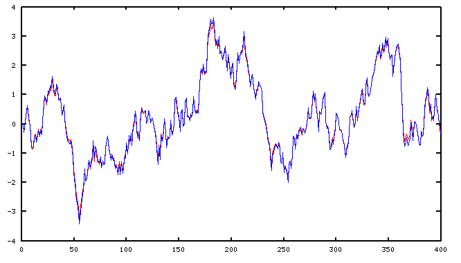
stato = zeros(4,1);
statn = zeros(4,1);
for istep=1:nsteps
  inp = rand-rand;
  yold(istep) = Cmat*stato;
  ynew(istep) = redC*statn;
  stato = Amat*stato + Bmat*inp;
  statn = redA*statn + redB*inp;
end

plot(1:nsteps,yold(1:nsteps),'r',1:nsteps,ynew(1:nsteps),'b')

The original system's response is the red curve. The reduced-order system response is the superimposed blue curve. There does not appear to be any serious damage or degradation. We could call this a success.

 

Identifying extraneous states

Let's think a little more about what kinds of states can be undesirable in a state transition model.

Unstable or marginally stable states

If the magnitude of a real or complex eigenvalue is greater than or equal to 1.0, the response is unstable or marginally stable. Is this something that you expected to be present in your model?

Extreme decay rate

If the magnitude of a real or complex eigenvalue is less than about 0.4 or so, the effects from this state fade to almost nothing in about 5 steps. For smaller eigenvalue terms, responses are gone before they have a chance to affect anything. This is not likely a behavior that you expect in the system, particularly if you have selected a reasonable sample rate, and a full cycle of any relevant frequency will be represented by a sequence of at least 10 samples.

Unexcited state (bad controllability)

In the almost-diagonal model, the state responses act independently. If the input coupling term for the state is unusually small, the response will be correspondingly small, and the state is probably meaningless.

Unobserved state (bad observability)

As we saw in our example, if states (or both of a complex pair of states) are associated with very tiny terms in the observation matrix, these states contribute almost nothing to the response and are not worth representing.

It might be worth checking for states are driven weakly and also observed weakly, so that in combination there is a very weak net contribution to the system output.

Redundant state

If two exponential states have very nearly the same eigenvalues, they produce very nearly the same net response. It is likely that you need only one of them. This is particularly true with Kalman filtering and states with very slow decay rates, because adjustments will override any tiny difference in the state behaviors.

 

Following up after order reduction

Reversing the transformation that was applied to near-diagonalize the state transition equations results in a set of equations as much as possible like the original equations, but of lower rank.

$$x_{i+1}=E\overline{\Lambda }{E}^{-1}{x}_i+E\overline{B}{u}_i$$ $$x_{i+1}=\overline{A}{x}_i+E\overline{B}{u}_i$$ $$y_{i+1}=\overline{C}{E}^{-1}{x}_{i+1}$$

However, there is still more to do, because the matrices remain the same sizes as before — clearly redundant. Next time, we will discuss the numerical housekeeping operations to clean up and finish the job.

 

---