Compacting the Reduced Model

In the previous installment, we identified states that were contributing nothing of significance to the state transition model, and cleared them away using a near-diagonal transformation of the system equations. While this reduced the order of the model, it left a state equation system of the original size. In this session, we will apply some numerical operations to clean out the redundancy, reducing the equation system to a minimal size.

 

The model deflation process

Start with the state equation systems in reduced order, as described in the previous installments, but still original size.

$$x^{1^{}}=A{x}^0+B{u}^0$$ $$y^1=C{x}^1$$

The value of the state vector x can be obtained by some linear combination of eigenvectors, since the set of eigenvectors is full rank. Let this particular combination of eigenvectors be described by vector q. Thus, we can define this particular decomposition as

$$x\equiv Eq$$

From the work that preceded, we know that the eigenvectors can be partitioned into two groups, the ones that have the original values, and the ones that are now associated with 0 eigenvalues (which is to say, they are orthogonal to all rows in the reduced A matrix). To help keep things organized, permute your variables (swap rows and columns in the eigenvalue and eigenvector matrices) to push all of the zero eigenvalues to the lower right, which correspondingly pushes the associated eigenvectors to the right.

After this reorganization, it is possible to partition the E matrix of eigenvectors to distinguish those having an influence on the system (the group E1) and those that do not (the group E0).

$$x=\left[\begin{array}{c}{E}_1{E}_0\end{array}\right]\left[\begin{array}{c}{q}_1\\ q_0\end{array}\right]$$

We can perform a similar analysis of the input coupling matrix B. This matrix can also be represented as a combination of the eigenvector terms. The particular combination that makes this happen can be defined as matrix V.

$$B=EV$$

As before, we can partition the V vector into the part V1 that the system state transitions responds to, and the part V0 that the state transition matrix does not respond to.

$$B=\left[\begin{array}{c}{E}_1{E}_0\end{array}\right]\left[\begin{array}{c}{V}_1\\ V_0\end{array}\right]$$

We can then observe that the next-state output can use the same eigenvector decomposition that was applied to the state vector within the state update formula. Applying all of these notation changes to the original state equations yields the following.

$$\left[\begin{array}{c}{E}_1{E}_0\end{array}\right][\begin{array}{c}{q}_1\\ q_0\end{array}{]}^1=A[\begin{array}{c}{E}_1{E}_0\end{array}\left]\right[\begin{array}{c}{q}_1\\ q_0\end{array}{]}^0+\left[\begin{array}{c}{E}_1{E}_0\end{array}\right]\left[\begin{array}{c}{V}_1\\ V_0\end{array}\right]u^0$$

Now we can apply some of the things we know about the state transition matrix and eigenvector properties to simplify. First, we know that when inputs produce new effects via the V0 matrix, these effects will go into the next state, but after that they will disappear in the very next state update, because the A matrix does not respond to them. This one-sample disturbance from input directly to output and then gone, is not a desirable feature to keep in the model. Set the V0 matrix terms to zero. (You might find that your previous order reduction steps have already forced the V0 matrix terms to zero, and if so, so much the better, because the disturbances are already gone!) In so doing, there is no longer any point in keeping the E0 matrix around, so the input coupling simplifies.

$$\left[\begin{array}{c}{E}_1{E}_0\end{array}\right][\begin{array}{c}{q}_1\\ q_0\end{array}{]}^1=A[\begin{array}{c}{E}_1{E}_0\end{array}\left]\right[\begin{array}{c}{q}_1\\ q_0\end{array}{]}^0+E_1{V}_1{u}^0$$

The result of multiplying the vectors in E0 times state transition matrix A yields only 0 vectors. Since these have no influence on next state, there is no point in keeping this vector or the corresponding q0 state terms around, so simplify again.

$$\left[\begin{array}{c}{E}_1{E}_0\end{array}\right][\begin{array}{c}{q}_1\\ q_0\end{array}{]}^1=A{E}_1{q_1}^0+E_1{V}_1{u}^0$$

Once the simplifications to the input coupling and the state transition terms are made, there is no remaining way for the q0 terms for next-state to have any value besides zero. There is no point in keeping these terms around. At this point, all of the E0 and q0 terms are gone from the reduced model.

$$E_1{q_1}^1=A{E}_1{q}_1+E_1{V}_1{u}^0$$

We have gotten rid of a lot of unnecessary terms, but not all of them. Believe it or not, we still have the same inflated number of state equations that we had originally. It is time to apply a surprising operator "out of the air." Define the following matrix.^[1]

$$M\equiv {\left({E_1}^T{E}_1\right)}^{-1}{E_1}^T$$

As strange as this might seem, it should not be completely unfamiliar. If you take a look at the classic Normal Equations^[2] solution to an overdetermined set of constraint equations for linear model coefficients, you will see a similar matrix combination in that context.

To see the motivation for this, take this unusual matrix and left-multiply every term in the state transition equation system.

$${\left({E_1}^T{E}_1\right)}^{-1}{E_1}^T{E}_1{q_1}^1={\left({E_1}^T{E}_1\right)}^{-1}{E_1}^{T}A{E}_1{q}_1+{\left({E_1}^T{E}_1\right)}^{-1}{E_1}^T{E}_1{V}_1{u}^0$$

That is really awful, but most of the terms result in inverse matrix terms that reduce to an identity, and can be removed.

$${q_1}^1={\left({E_1}^T{E}_1\right)}^{-1}{E_1}^{T}A{E}_1{q}_1+V_1{u}^0$$

One term remains messy, but since it involves only the matrix terms E1 and A, it is really not particularly difficult to compute.

One more detail. The original state vector x can be expressed in terms of the eigenvectors as it was in the state transition equations.

$$y=Cx=CEq$$

Since the q0 terms are zero and play no role anywhere else, we can make the corresponding simplification here. So this completes the reduced model.

$$y=C{E}_1{q}_1$$

 

The test

Let us apply these equations, starting from the reduced order but oversize model that we had previously. Observe that the two zero-valued eigenvalues are located at the lower right.

redA =
   7.8003e-01   4.6840e-01  -4.2817e-01   4.4327e-01
  -1.3154e-17   7.8000e-01  -2.4131e-17   1.9392e-17
  -6.7964e-01   8.5388e-01   3.7307e-01  -3.8622e-01
  -3.1662e-01   3.8693e-01   1.7380e-01  -1.7993e-01

redB =
   0.37488
   1.00000
   1.29131
   0.58764

redC =
   0.88789  -0.65062  -0.48738   0.50456

eigval =
   0.97317   0.00000   0.00000   0.00000
   0.00000   0.78000   0.00000   0.00000
   0.00000   0.00000  -0.00000   0.00000
   0.00000   0.00000   0.00000   0.00000

The active eigenvectors are then easily extracted from the leftmost columns of the eigenvector matrix.

E1 =
   0.72095  -0.20947
   0.00000   0.39068
  -0.62816   0.81460
  -0.29264   0.37405

The reduced system is calculated according to the methods described above.

   E1 = eigvec(:,1:2)
   VV = eigvec^-1 * redB;
   V1 = VV(1:2)
   MINV = (E1' * E1)^-1;
   Qmat = (E1' * redA * E1);
   Ra = MINV*Qmat
   Rb = V1
   Rc = redC*E1

 
V1 =
   1.2637
   2.5597

Ra =
   9.7317e-01   3.0293e-16
   3.2960e-17   7.8000e-01

Rb =
   1.2637
   2.5597

Rc =
   0.79863  -0.64846

As a sanity check, the eigenvalues of the final reduced matrix are checked.

eigenvalues =
   0.97317
   0.78000

This all looks pretty good, but let's see if the system behaves the same when driven with random data.

stato = zeros(4,1);
statn = zeros(2,1);
for istep=1:nsteps
  inp = rand-rand;
  yold(istep) = redC*stato;
  ynew(istep) = Rc*statn;
  stato = redA*stato + redB*inp;
  statn = Ra*statn + Rb*inp;
end

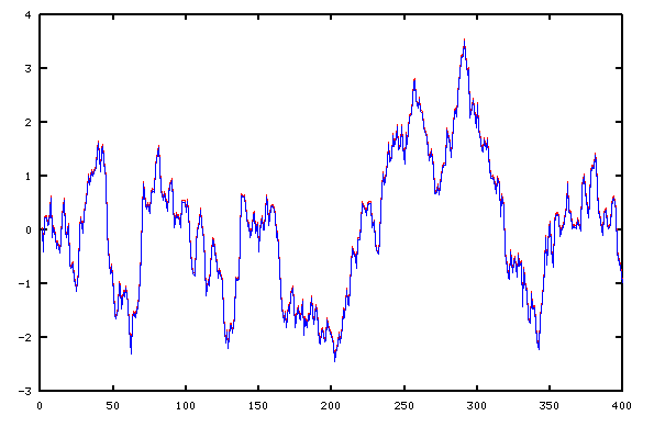
Actually, I had to cheat. Without fudging the graphics by shifting the red curve a couple of pixels, the tracking was so perfect that the two traces were completely indistinguishable.

 

A retrospective

Let's briefly review how far we have come. If you have followed this series from the beginning:

1. You can apply Linear Least Squares or Total Least Squares methods to fit the parameters of a linear state transition model.
2. You can compare how your model predictions perform compared to actual system outputs by simulation.
3. You can restructure models that require multiple steps of past history into models requiring only one step of past history and multiple state variables using shift register techniques.
4. You can transform ARMA models developed using statistical methods into equivalent state transition models.
5. You can improve your models numerically, using LMS gradient learning techniques.
6. You can apply scaling, transposition, restructuring, and eigenvalue transformations to change the form of the state transition matrix without changing its performance.
7. You can use correlation analysis to check whether your model captures all of the important behaviors of the system and to deduce an appropriate model order.
8. You can adjust your model order by learning new response characteristics or removing insignificant ones.

All of these techniques take an adaptive systems approach to modeling. That is: assume that your system model needs to be improved to make it match the real system more closely. That is surely the case when you start with no model at all!

When you reach the point that your state transition equations give rather credible but imperfect tracking of the real system behavior, it is time to change gears and consider the Kalman Filter approach. We know that the model results are going to be imperfect, because the real system has noise disturbances that the model does not and cannot know about. The random disturbances propagate in the state variables to send the system along a different trajectory than the model predicts.

We can't be completely sure at any individual point what the noise effects are, but over a longer period, we can start to see systematic trajectory changes. When we see those, we can be increasingly confident that they resulted from random effects, and we can take action to restore accurate tracking. We begin this new direction next time.

 

---