Another page [1] on this site describes how to design min-max "Chebyshev-optimal" filters to calculate numerical estimates of the first derivative from sampled data. This page extends that approach to estimate the second derivative. Despite highly useful results, the designs are not necessarily the best choice for all applications.
Adapting the solution method
While the approach used for designing first-derivative approximators applies nicely, there are several details to take into account to apply the same approach to second-derivative approximators.
-
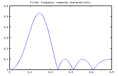
Filter response characteristic. Since the second derivative estimator is the equivalent of applying a first-derivative estimator twice, the frequency-domain response of the second-derivative filter will be the equivalent of two multiplications by
wand two phase shifts byΠ/2. Thus, in the critical low-frequency region, the response curve is an upward-bending quadratic curve. The combination of the two phase shifts is the equivalent of multiplying by a scalar factor-1.0. This is a somewhat harder problem numerically because the upward curvature must be countered by downward curvature to return the response curve somewhat close to zero at high frequencies, thus avoiding excessive noise response. The filters tend to need a few more terms than the first-derivative approximators to achieve similar accuracy. -
Basis functions. A second derivative filter will have even symmetry. Cosine waves have the desired properties. So, instead of using a sine-series approximation as in the first-derivative case, use a cosine series approximation.
-
No natural zero constraint. The second derivative of a constant sequence is zero, much like the first derivative. However, cosine "basis functions" do not have a natural property of passing through zero. Thus, a constraint that the combination of cosine functions must equal 0 at 0 frequency must be included, with rigorous tolerance on this requirement. Since the value of a cosine function is 1.0 when evaluated at 0, this constraint is equivalent to saying that the sum of the filter coefficients must be equal to 0.
-
Basis size. The number of terms in each of the basis vectors of matrix
BisN/2 - Ntterms rather thanN/2 - 1 - Ntterms, to account for the added constraint at location 0.
After taking these adjustments into account, the solution method is fundamentally the same as for the first-derivative case. Full details of the method are provided on the page that covers the first-derivative case [1].
Here is the result of a typical design (see the 15-term design below).
Design script
An m-file design script for Octave shows the numerical details of constructing the matrix terms, calculating the solution, and plotting the results for the second-derivative filter design. If you wish to experiment with this script, download a copy of the minmax2.m file. The Octave solution is based on the GLPK package, but you can use the equivalent solver from the Optimization Toolbox for Matlab [2].
Comparison to other designs
To see the practical benefits of the min-max designs, the 15-term filter (as tabulated below) is compared to the 9-term "Robust Low Noise" (RLN) design from Pavel Holoborodko's site. While this comparison seems inherently unfair — the min-max design is allowed 60% more parameters to work with — this is the best we can do.
-
The ninth-order RLN design is the highest order filter listed.
-
The RLN designs in general deliver less accuracy as the filter order increases, except near zero frequency, as you can clearly see from the frequency response plots for estimators of various orders. More parameters only makes the comparison more unfair.
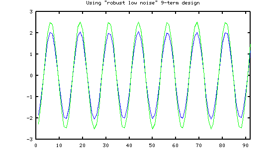
First, here is the performance delivered by the RLN method in the presence of white random noise at 5% of the signal level, at a frequency of about 8% of the sampling rate (approximately 12 terms span a complete waveform cycle). A mathematically perfect result in green is plotted on top of the filter estimates in blue.
Next, here is the performance delivered by the min-max method, same level of random noise and signal. (The apparent different number of terms is only an artifact of the differing filter length.)
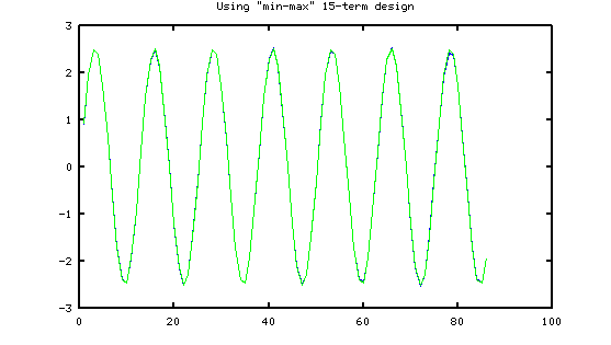
It might seem like the min-max design is an undisputed winner — but unfortunately, the choice is not that clear. While the min-max design tracks changing curvature and higher frequencies better, the "RLN" approach concentrates maximum effort at matching low frequencies accurately, and does this with great efficiency.
Some tabulated results
The following table provides some design results that you can use directly without resorting to the design script. For each target number of filter terms, the design parameters, the resulting performance specs, and filter coefficients are listed. If you are not sure about where to start, try the 15-term filter design with its 0.08·Fs guaranteed accurate band. If you need more economy or better performance, switch to one of the other designs.
| 11-term — 5% accurate — 8% useful |
| Design: pass: 0.05 transition: 0.185 sensitivity: 100.0 |
| pass ripple: 0.001 stopband edge: 0.24 stopband ripple: 0.10 |
filter: -0.024705 0.064369 0.070200 0.018820 -0.070707 -0.115954 -0.070707 0.018820 0.070200 0.064369 -0.024705
|
| 13-term — 6% accurate — 9% useful |
| Design: pass: 0.08 transition: 0.135 sensitivity: 100.0 |
| pass ripple: 0.001 stopband edge: 0.21 stop ripple: 0.104 |
filter: -0.0303998 0.0062139 0.0870660 0.0549440 0.0219066 -0.0862821 -0.1068973 -0.0862821 0.0219066 0.0549440 0.0870660 0.0062139 -0.0303998
|
| 15-term — 8% accurate — 11% useful |
| Design: pass: 0.08 transition: 0.14 sensitivity: 150 |
| pass ripple: 0.00075 stopband edge: 0.22 stopband ripple: 0.1 |
filter: 0.010053 -0.051074 0.018345 0.070910 0.081264 0.017178 -0.081808 -0.129738 -0.081808 0.017178 0.081264 0.070910 0.018345 -0.051074 0.010053
|
| 17-term — 10% accurate — 13% useful |
| Design: pass: 0.10 transition: 0.16 sensitivity: 420 |
| pass ripple: 0.0002 stopband edge: 0.26 stopband ripple: 0.082 |
filter: -0.0020745 0.0274629 -0.0434860 -0.0404178 0.0523018 0.1458368 0.0842230 -0.1122293 -0.2232337 -0.1122293 0.0842230 0.1458368 0.0523018 -0.0404178 -0.0434860 0.0274629 -0.0020745
|
Footnotes:
[1] The page on this site about first-derivative filter approximation has the details about to set up and solve the approximation problem.
[2] The "robust low noise estimators" are described at Pavel Holoborodko's web site, http://www.holoborodko.com/pavel/numerical-methods/numerical-derivative/smooth-low-noise-differentiators/.
[3] You can find more information about the Optimization Toolkit at
http://www.mathworks.com/products/optimization/index.html .