What is optimal exactly?
Other sites:
Being optimal has everything to do with what exactly you are attempting to optimize.
In the case of numerical differentiators, optimal will mean that that the filter is of minimum length in order to achieve a sufficient degree of accuracy at low frequencies where the numerical estimates matter, but with a sufficient rejection of high frequency noise. It is likely that the high frequency noise components are already relatively small in the original data, so it is not really necessary to drive the frequency response vigously to zero, as occurs in asymptotic or frequency-domain designs. All you need to do is attenuate the noise rather than amplify it.
If you don't care about the theory but just want some results to try, skip to the filter table at the end of this page. Or if you need a second derivative estimator, try the results presented at the end of the second derivative page.
Review
To briefly review the background material from other pages on this site [1] and elsewhere [2][3], the problem is to devise a filter to estimate the first derivative of a function from samples of that function. Classical methods based on such methods as finite difference and polynomial approximation promise very high accuracy, but they tend to perform poorly in practice because of extreme sensitivity to high frequency noise. That makes them a relatively poor choice when the samples are obtained by measurement.
For a given function f(t) with Fourier transform F(jw),
the transform of its derivative is jw·F(jw). That is, a derivative
operator changes the original spectrum by "phase shifting it" by angle pi/2
and multiplying it by the frequency w. (In the simple case of a sine
function, sin'(wt) = w·cos(wt) = w·sin(wt + Π/2) so
the phase shift and scaling are particularly obvious.) Since a convolution filter
in the time domain is a multiplication in the frequency domain, we can obtain a
time domain filter that approximates a derivative operation if the transform of
this filter has a magnitude response w and a phase shift
Π/2. The transform of a sine function has the desired phase and
symmetry properties, and similar for a sum of sine functions, so a reasonable
strategy for obtaining the filter is to approximate the amplitude response
function f(w) = w using a finite sine function series over a
reasonable frequency range. For a set of sine functions at equally spaced discrete
frequencies, we know from Discrete Fourier Transform properties that the coefficients
of the sine function terms will yield the coefficients for the desired
convolution filter.
The original functions or signals from which samples are taken must not have frequencies higher than 1/2 the sample rate — the theoretical "Nyquist Limit" — otherwise information is lost during sampling, as high frequencies and low frequencies become indistinguishable in the sampled data set. At the frequency limit, there are only two samples present in each wave cycle. In practice, it is difficult to extract useful information from very sparsely sampled data sequences near the limit, even if the theoretical restrictions are satisfied. So it is advisable to sample in such a manner that every meaningful up-down pattern in the sampled data set is spanned by at least 10 samples — 10% or less of the sampling rate, 20% or less of the theoretical Nyquist frequency limit. Any remaining higher-frequency effects can then be considered extraneous noise.
Ordinarily, because of its increasing gain at high frequencies, a derivative
estimator strongly amplifies high-frequency noise. To avoid this excessive gain,
a desirable derivative estimator will deviate from the f(w) = w curve
at high frequencies, and instead of amplifying high-frequency noise it will
attenuate the noise significantly. It is not necessary to totally eliminate all
high frequency noise, however, since a good data set will start with only a
limited amount of high frequency noise.
Other solutions
Classical Divided Difference methods are very bad because of high frequency noise amplification; this approach is suitable only with mathematically perfect data.
A naive Least Squares approach to fitting a derivative filter by polynomial methods is better, but limited and offering no clear means of improvement.
A low noise derivative estimation filter using a max flat filter characteristic is described by Pavel Holoborodko [3]. A max flat filter is one for which there is a high degree of tangency to the desired response curve at frequency 0, and also a high degree of tangency to a flat zero-response line at the Nyquist frequency limit.
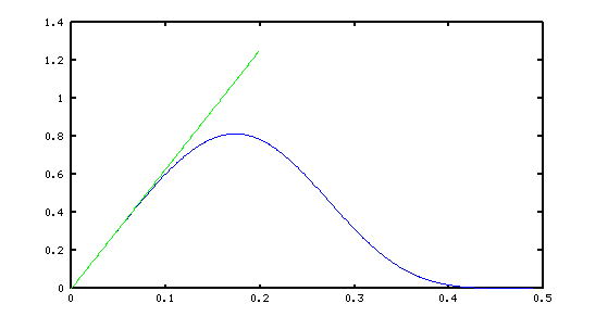
This is an interesting idea yielding an economical design, but with
some of drawbacks. It provides no real control over the accuracy. While
the design illustrated approximates the desired f(w) = w curve
sufficiently through about 0.03 or so of the sampling rate, it continues to respond,
inaccurately, through a relatively wide range, at a relatively high level
through about 0.30 of the sampling rate.
FFT-based designs presented on this site are based on sine-series approximation, and they produce very accurate filter characteristics with aggressive rejection of high frequency noise, such as the following:
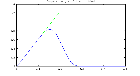
The FFT-based filter designs look very good. Based on a signal with peak magnitude 1.0, the accuracy in the low frequency band is within approximately ±0.0001, maintaining this accuracy through the entire useful band, yet transmission of noise is negligible beyond approximately 0.25 of the sampling rate. Comparing the "low noise" and "frequency domain" designs like this is rather unfair, however, since the attractive properties of the FFT-based designs do not come cheaply: many more filter coefficients are required.
The optimal design described on this page attempts to approximate the derivative filter characteristic vigorously at the low frequencies, where accuracy is critical, while allowing pretty much anything at other locations as long as the noise that leaks through at high frequencies is acceptably bounded. The term "optimal" as used here in the sense of the "Chebyshev criterion" — the maximum deviation from the ideal response specification is minimized. The result is an approximation that enforces accuracy where needed, but with considerably more computational efficiency than FFT designs.
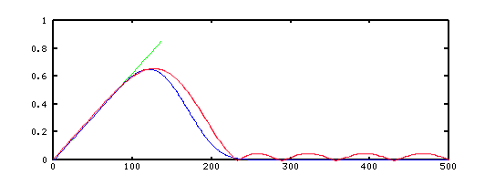
The following graphic compares the characteristics of a typical optimal estimator with an estimator designed by FFT methods. The FFT design, shown in blue, is approximately the same in the important low-frequency "passband" region, just a little better in the transition between the desired low-frequency band and the high frequencies, and a little quieter in the "stopband" region. The optimal design, shown in red, matches remarkably well, considering that the FFT design used 25 filter terms, while the optimal design uses 13.
Characterizing an Optimal Differentiator Design
A min-max optimal derivative approximation filter is described by the following design parameters:
-
The number of sine functions
Nfto use for the approximation.
Since the filters will have odd symmetry, and the center term is always 0.0, only half of the coefficients are calculated, and then the rest constructed by symmetry. The number of terms in the designed filter is then2·Nf+1. A filter with more terms requires more computation, but in general yields better accuracy, with tighter control on the size of the deviations, the transition region width, and so forth. The portion of the frequency band that must be fit accurately.
Express it as a fraction of the sampling frequency. Typical range:0.05 to 0.15. A shorter band typically allows a faster transition with less low-frequency noise, but typically allows much more high frequency noise to pass.-
The portion of the frequency band that is unrestricted.
This "transition region," between the band to fit accurately and the band to bound near zero, is uncontrolled. Fortunately, sine series approximations tend to be relatively well-behaved in this region. The transition band is also specified as a fraction of the sampling frequency. Typical range:0.10 to 0.30. A narrow region allows less low-frequency noise to pass, but typically with a side effect of allowing more noise to pass through at higher frequencies. -
The passband sensitivity factor.
This specifies a desired ratio of peak noise leakage "ripple" in the high frequency "stopband" to the peak fit errors in the low frequency "passband." A typical value is 50 to 2000. A large factor yields a closer approximation at the important low frequencies, with more noise passing through at high frequencies. You can't directly specify the size of approximation errors, but you can use this ratio to seek a suitable compromise.
Outline of the Optimal Design Method
The designed filter characteristic will consist of a best weighted sum of "basis functions," each of which is a sine wave of a different frequency. While ideally each sine wave is evaluated at every possible point along the wave, we can get a very close and practical approximation by evaluating each wave at some sufficiently large number N discrete points. A typical value of N might be approximately 400 to 1000. To be consistent with a Fourier analysis, the first selected frequency for the sine function series covers one sine-wave cycle in these N points. The frequency of the second sine function covers two complete waveform cycles in these N points, and so forth, for each of the Nf frequencies.
Identify the number of terms that should be retained in the basis vectors.
Because of symmetry properties, half of the
Npoints along each sine wave are redundant. The secondN/2terms are dropped without losing any information.We can leave out the first "zero term" because sine waves are always equal to zero at argument value zero — and so is the derivative. We don't need to apply a constraint to obtain an exact match.
Identify terms that correspond to low frequencies where the derivative filter must fit accurately. To obtain a filter that approximates well through frequency
0.1of the sampling frequency, for example, chooseNp = N · 0.1, roundingNpup or down to the nearest integer.Terms corresponding to the unrestricted transition region between the low "passband" frequencies and the high "stopband" frequencies are skipped. For example, if a transition region of width
0.12is allowed, then the nextNt = N·0.12terms are omitted.Any remaining terms beyond the transition zone correspond to high frequencies where little noise should pass through.
Thus, the basis vectors include N/2 - 1 - Nt terms. Collect the basis vectors to form a very long, narrow matrix B.
Now we can consider the desired response curve. In the "accurate low frequency band," the "ideal derivative response" should be matched.
b(k) = 2 Π k / N for k = 1 to Np
We would like all of the remaining N/2 - 1 - Nt - Np terms of vector b to be zero, so that under perfect conditions no noise passes through.
If our sine functions just happened to combine to produce a perfect result, there would exist the solution vector x of coefficients such that the following overdetermined matrix constraint is satisfied exactly.
B x = b
But we cannot expect this kind of exact match. We can introduce a tolerance vector T consisting of all 1 terms, and a "deviation" variable m to multiply this. This extra term represents a "tolerance" that bounds the worst case approximation error. By making m sufficiently large and positive we can establish the condition that
B x + T m - b ≥ 0
In a similar manner, we could subtract T in such a way that the following constraint is satisfied.
B x - T m - b ≤ 0
Letting I represent an identity matrix of appropriate rank, it is possible to introduce positive "slack variables" s1 and s2 into each constraint to "make up the difference" so that equality holds, converting the above inequality constraints into equality constraints on positive variables.
B x + T m - b - I s1 = 0
B x - T m - b + I s2 = 0
The multipliers on the B matrix columns are not constrained to be positive, however. To recast the constraints so that a sign restriction does hold, we can split each coefficient in solution x into two parts, xm and xp, such that the solution variable is x = xp - xm and where both xm and xp are non-negative but at least one is equal to 0. Then all of the variables are constrained to be non-negative.
B xp + -B xm + T m - I s1 = b
B xp + -B xm - T m + I s2 = b
Scaling the first equation on both sides, and doing a little rearrangement of terms, we can get an equivalent set of constraints expressed in matrix form.
      M   X    =   V

   with
       M  =   | -B   B   -T    I   0  |
              |  B  -B   -T    0   I  |

       V  =   | -b  |
              |  b  |

       X  =   |  xp  xm  m  s1  s2  |'

       T  =   |  1   1   1  ...  1  |'
where the solution vector X is to be determined such that all
of the constraints are satisfied, and all of the X terms are nonnegative.
If variable m is set positive and equal to the largest positive term in vector V, this is sufficient to force the M·X product to be non-positive in every row. Thus, non-negative values for the s1 and s2 variables can be applied to satisfy every constraint conditions. This yields a candidate solution that satisfies the matrix constraints, and also satisfies the sign constraints on all variables. Thus, it is very easy to establish a a feasible candidate solution that satisfies both the constraint equations and the sign conditions.
However, since the xm and xp variables that we want to determine play no part in this yet, the initial candidate solution is clearly not a useful solution to the problem. A good solution would satisfy all constraint and sign conditions, but with the value of m as small as possible, and with the weighted sum of the sine functions matching the b values as close as possible. Thus, the filter coefficients are obtained by minimizing m such that none of the matrix or sign constraints are violated. This sounds complicated... but it turns out that Danzig's classic "Simplex LP" algorithm can solve this problem easily.
One last important detail. As formulated above, the designs will show equal deviations from the desired ideal shape both at high frequencies where variations of a few percent don't matter, and at low frequencies where a high degree of accuracy is critical. To correct this serious deficiency, modify the terms in the T vector that correspond to 0 values of the b vector by replacing the previous value of 1.0 with the sensitivity factor design parameter value. Since this "sensitivity factor" is typically much larger than 1, a small adjustment in the m variable allows much larger deviations from the ideal in the high frequency band "at little cost," while the solution must maintain tight accuracy at the critical low frequencies.
Design script
The m-file design script for Octave shows the numerical details of constructing the matrix terms, calculating the solution, and plotting the results. This formulation uses inequality constraints rather than equality constraints, so the s1 and s2 variables are not used explicitly. If you wish to experiment with this script, download a copy of the minmax.m file. The Octave solution is based on the GLPK package, but you can use the equivalent solver from the Optimization Toolbox for Matlab [5] at a price.
On the other hand, if you need a filter design to use immediately, without all of the complications of doing your own designs, see the next section.
Some tabulated results
The following table provides some design results that you can use directly without resorting to the design script. For each target number of filter terms, the design parameters, the resulting performance specs, and filter coefficients are listed. If you are not sure about where to start, try the 11-term filter design with 0.07·Fs guaranteed accurate band. If you need
more economy or better performance, switch to one of the other designs.
| 9-term — 4% flat — 6% useful |
| Design: pass: 0.042 transition: 0.22 sensitivity: 1.0 |
| pass ripple: 0.007 stopband edge: 0.21 stopband ripple: 0.007 |
filter: -0.023422 -0.059950 -0.084427 -0.063318 0.000000 0.063318 0.084427 0.059950 0.023422
|
| 9-term — 8% flat — 10% useful |
| Design: pass: 0.085 transition: 0.32 sensitivity: 1.0 |
| pass ripple: 0.001 stopband edge: 0.36 stop ripple: 0.001 |
filter: 0.02827 0.01063 -0.17942 -0.28242 0.00000 0.28242 0.17942 -0.01063 -0.02827
|
| 11-term — 4% flat — 7% useful |
| Design: pass: 0.04 transition: 0.18 sensitivity: 500 |
| pass ripple: 0.00025 stopband edge: 0.19 stopband ripple: 0.14 |
filter: 0.03702 -0.01141 -0.09121 -0.12991 -0.10528 0.00000 0.10528 0.12991 0.09121 0.01141 -0.03702
|
| 11-term — 7% flat — 10% useful |
| Design: pass: .0725% transition: 0.17 sensitivity: 100 |
| pass ripple: 0.001 stopband edge: 0.24 stopband ripple: 0.10 |
filter: 0.01596 0.04073 -0.09074 -0.16089 -0.14287 0.00000 0.14287 0.16089 0.09074 -0.04073 -0.01596
|
| 13-term — 7% flat — 10% useful |
| Design: pass: 0.07 transition: 0.16 sensitivity: 650 |
| pass ripple: 0.0002 stopband edge: 0.24 stop ripple: 0.10 |
filter: -0.02714 0.06757 0.02006 -0.08312 -0.17684 -0.15134 0.00000 0.15134 0.17684 0.08312 -0.02006 -0.06757 0.02714
|
| 13-term — 12% flat — 14% useful |
| Design: pass: .012 transition: .175 sensitivity: 200 |
| pass ripple: 0.0006 stopband edge: 0.30 stop ripple: 0.13 |
filter: -0.00298 -0.02798 0.08970 0.00543 -0.22013 -0.28016 0.00000 0.28016 0.22013 -0.00543 -0.08970 0.02798 0.00298
|
| 15-term — 8% flat — 11% useful |
| Design: pass: .08 transition: .165 sensitivity: 1150 |
| pass ripple: 0.00009 stopband edge: 0.24 stop ripple: 0.10 |
filter: -0.00010 -0.02786 0.05824 0.03528 -0.07183 -0.18890 -0.17186 0.00000 0.17186 0.18890 0.07183 -0.03528 -0.05824 0.02786 0.000108
|
Footnotes:
[1] A page on this site provides background information about the general problem of designing numerical derivative estimators, with focus on second-derivative filters. Some design methods are discussed that seemed promising but proved to be less effective.
[2] The classic "Digital Filters" by R. W. Hamming covers the derivative estimator filters from a frequency analysis point of view. The FFT method (reference 4 below) is an elaboration of the ideas presented there.
[3] You can find Pavel Holoborodko's pages on derivative filter approximation at
http://www.holoborodko.com/pavel/numerical-methods/numerical-derivative/smooth-low-noise-differentiators/. This is one of the better sources of information about central differences and other design methods for derivative filter designs.
[4] A page on this site discusses designing filters using FFT methods. It it tricky to set up a design. Applying these filters requires extra computation, but otherwise the results seem about as good as you can get.
[5] You can find more information about the Optimization Toolkit at
http://www.mathworks.com/products/optimization/index.html .